Using Matlab code to compute and compare errors in Central differencing, Skewed forward and Skewed backward methods of a second derivative through Taylor's Table method.

In this program, the error values of the second derivative of the function `e^x*cos(x)` are calcluated by using 3 different methods. These methods are central differencing, skewed forward and skewed backward methods. The approximation considered for all these methods are fourth order as given in the problem statement.

• Central differencing method

In this method, the stencil considered for calculation is symmetric. In this problem the number of nodes for central differencing method is calculated to be 5. The numerical stencil is as represented below:

-----()-------()---------()----------()----------()

f(i-2) f(i-1) f(i) f(i+1) f(i+2)

The coeffiecients are evaulated by using taylor series method and are obtained by using matrix inversion method in matlab. The below table indicates the taylor table for this method. Further this table was deduced into matrix form and solved in matlab. Then these values were used to compute the numerical error value.

Terms	f(i)	f'(i)*dx	f^2(i)*dx^2	f'''(i)*dx^3	f^4(i)*dx^4	f^5(i)*dx^5
a*f(i-2)	a	-2a	2a	-8a/6	16a/24	-32a/120
b*f(i-1)	b	-b	b/2	-b/6	b/24	-b/120
c*f(i)	c	0	0	0	0	0
d*f(i+1)	d	d	d/2	d/6	d/24	d/120
e*f(i+2)	e	2e	2e	8e/6	16e/24	32e/120

• Skewed right sided difference

In this method, the numerical stencil is considered to right side of the point of the function for approximation. The number of nodes calculated for the given problem is 6. The stencil is as represented below and similar to the above method, first a taylor table is built and then is converted into a matrix, which is solved in matlab.

-------()--------()---------()--------()---------()----------()

f(i) f(i+1) f(i+2) f(i+3) f(i+4) f(i+5)

The coeffiecients are calculated in a similar manner to the above method and are used to compare error. The taylor table is as shown below

Terms	f(i)	f'(i)*dx	f^2(i)*dx^2	f'''(i)*dx^3	f^4(i)*dx^4	f^5(i)*dx^5
a*f(i)	a	0	0	0	0	0
b*f(i+1)	b	b	b/2	b/6	b/24	b/120
c*f(i+2)	c	2c	2c	8c/6	16c/24	32c/120
d*f(i+3)	d	3d	9d/2	27d/6	81d/24	243d/120
e*f(i+4)	e	4e	8e	64e/6	256e/24	1024e/120
f*f(i+5)	f	5f	25f/2	125f/6	625f/24	3125f/120

• Skewed backward difference:

The methods used to solve are similar to above discussed methods, only the direction of numerical stencil is reversed. The nodes considered are backward from the actual point of function. Again for this method the nodes are calculated to be 6. The stencil is shown below:

-----()------()-------()--------()-------()-------()

f(i-5) f(i-4) f(i-3) f(i-2) f(i-1) f(i)

Overall the formulae used to calculate the number of nodes are:

For asymmetric stencil, Order of Approximation = Number of nodes in the stencil - Order of the Derivative

For symmetric stencil, Order of Approximation = Number of nodes in the stencil - Order of the Derivative + 1

Taylor table used for this method remains the same, the only difference is that while writing the code, the odd coefficients in should be made negative. The table is as shown below:

Terms	f(i)	f'(i)*dx	f^2(i)*dx^2	f'''(i)*dx^3	f^4(i)*dx^4	f^5(i)*dx^5
a*f(i)	a	0	0	0	0	0
b*f(i+1)	b	b	b/2	b/6	b/24	b/120
c*f(i+2)	c	2c	2c	8c/6	16c/24	32c/120
d*f(i+3)	d	3d	9d/2	27d/6	81d/24	243d/120
e*f(i+4)	e	4e	8e	64e/6	256e/24	1024e/120
f*f(i+5)	f	5f	25f/2	125f/6	625f/24	3125f/120

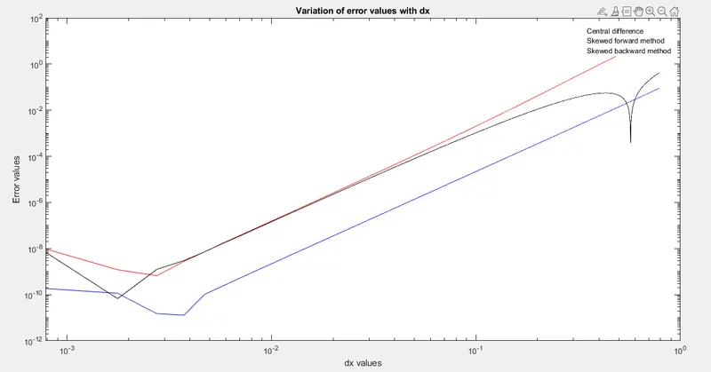
• All the above discussed methods are used determine error value wrt changes in dx values. The range of dx values considered for this problem are [pi/4,pi/4000,800]. Value of x is considered to be pi/3. More number of values are considered to get good graphical representation.
• An additional point is that, while computing in my system due to software problems, I was not able to get the legend representations. It is possible to get them in another system. For the same reason, legend is not proper in the screenshot provided below.

Matlab program:

function error = second_order_derivative_approximation(x)

dx = linspace(pi/4,pi/4000,800);%The range of values for which the calculation is carried out. More number of values are taken to get a good graph.

%% These are the matrices of central differencing method.
Main_matrix_CD = [1 1 1 1 1; -2 -1 0 1 2;2 1/2 0 1/2 2;-4/3 -1/6 0 1/6 4/3;16/24 1/24 0 1/24 16/24];%This is the main matirx indicating the co-effiecients of different derivatives
%Number of nodes are calculated to be 5, hence the matrix dimensions are
%5*5.
Sub_matrix_CD = [0;0;1;0;0];%This matrix represents that only the second order derivative is evaluated.

CD_method = inv(Main_matrix_CD)*Sub_matrix_CD;%Inverse funtion is used to calculate the value of coefficients.

%% Skewed forward differencing method.
Main_matrix_SKF = [1 1 1 1 1 1;0 1 2 3 4 5;0 1/2 2 9/2 8 25/2;0 1/6 8/6 27/6 64/6 125/6;0 1/24 16/24 81/24 256/24 625/24;0 1/120 32/120 243/120 1024/120 3125/120];%Main matrix for Skewed forward differencing method.

Sub_matrix_SKF = [0;0;1;0;0;0];%The number of nodes are calculated to be 6. So there are 6 columns in this matrix and 6 rows and columns in the previous matrix.

Skewed_forward_difference = inv(Main_matrix_SKF)*Sub_matrix_SKF;

%% Skewed backward differencing method.

Main_matrix_SKB = [1 1 1 1 1 1;0 -1 -2 -3 -4 -5;0 0.5 2 9/2 8 25/2;0 -1/6 -8/6 -27/6 -64/6 -125/6;0 1/24 16/24 81/24 256/24 625/24;0 -1/120 -32/120 -243/120 -1024/120 -3125/120];
%The above matrix dimension of 6*6 indicates the number of nodes to be 6.
Sub_matrix_SKB = [0;0;1;0;0;0];

Skewed_backward_difference = inv(Main_matrix_SKB)*Sub_matrix_SKB;%% 

%% Calculation of the value of second order derivative in both analytical and numerical methods.

analytical_function = -2*exp(x)*sin(x);%This is second order derivative of exp(x)*cos(x).The value of x is considered to be pi/3.

for i = 1:length(dx)%for loop is used to go through every value of dx and calculate the numerical and error values for the given function.
        
    central_differencing_Scheme(i) = ((CD_method(1)*exp(x-(2*dx(i)))*cos(x-(2*dx(i))))+(CD_method(2)*exp(x-dx(i))*cos(x-dx(i)))+(CD_method(3)*exp(x)*cos(x))+(CD_method(4)*exp(x+dx(i))*cos(x+dx(i)))+(CD_method(5)*exp(x+(2*dx(i)))*cos(x+(2*dx(i)))))/(dx(i)^2);
    %Central differencing method uses symmetrical stencil for calculation.
    skewed_forward_Differencing(i) = ((Skewed_forward_difference(1)*exp(x)*cos(x))+(Skewed_forward_difference(2)*exp(x+dx(i))*cos(x+dx(i)))+(Skewed_forward_difference(3)*exp(x+(2*dx(i)))*cos(x+(2*dx(i))))+(Skewed_forward_difference(4)*exp(x+(3*dx(i)))*cos(x+(3*dx(i))))+(Skewed_forward_difference(5)*exp(x+(4*dx(i)))*cos(x+(4*dx(i))))+(Skewed_forward_difference(6)*exp(x+(5*dx(i)))*cos(x+(5*dx(i)))))/(dx(i)^2);
    %Skewed forward method utilizes 6 forward nodes for calculation.
    skewed_backward_Differencing(i) = ((Skewed_backward_difference(1)*exp(x)*cos(x))+(Skewed_backward_difference(2)*exp(x-dx(i))*cos(x-dx(i)))+(Skewed_backward_difference(3)*exp(x-(2*dx(i)))*cos(x-(2*dx(i))))+(Skewed_backward_difference(4)*exp(x-(3*dx(i)))*cos(x-(3*dx(i))))+(Skewed_backward_difference(5)*exp(x-(4*dx(i)))*cos(x-(4*dx(i))))+(Skewed_backward_difference(6)*exp(x-(5*dx(i)))*cos(x-(5*dx(i)))))/(dx(i)^2);
    %Skewed backward method uses 6 backward nodes for calculation.
    
    error_central(i) = abs(analytical_function-central_differencing_Scheme(i));%This indicates the error value between analytical and central differencing method.

    error_skewed_forward(i) = abs(analytical_function-skewed_forward_Differencing(i));%This indicates the error value between analytical and skewed forward method.
    
    error_skewed_backward(i) = abs(analytical_function-skewed_backward_Differencing(i));%This calculates the error value between analytical and skewed backward method.
    
end

loglog(dx,error_central,'b')%loglog function is used plot the graph in a large scale and also to match the different set of values in a single graph
hold on%This function is used to solve plot multiple curves on the same plot.

loglog(dx,error_skewed_forward,'r')%plots the skewed forward method errors
loglog(dx,error_skewed_backward,'k')%plots the skewed backward method erros
%labelling the graph
xlabel('dx values')
ylabel('Error values')
title('Variation of error values with dx')
legend('Central difference','Skewed forward method','Skewed backward method')%The legend used here is correct, but due to the software issues, the representation is absent and hence it cannot be seen in the screenshot. For confirmation please run the program.

end

Screenshot:

Result explanation:

• From the formula, The order of accuracy P = Number of nodes in the stencil N - order of derivative Q, where for skewed scheme, number of nodes are 6 and the order of derivative is 2, The order of accuracy obtained is 4. This is also verified by comparing in the derivation, where the lead term in truncation error is of fourth order.

• It is evident from the graph that, central differencing scheme has the least error values throughout the range of dx.

• Compared to central differencing method, skewed methods provide lesser accurate results. But in the case of convection diffusion problems, the accuracy is less compared to skewed methods. Since central differencing method considers points behind and ahead of the actual point, this is applicable in case of a boundary which is continuous.

• When a boundary is considered, to solve central differencing method, nodes beyond the boundary cannot be considered. Skewed forward and backward methods help to solve the problem in this case. This is why skewed methods are important.