Challenge

Channel flow simulation using CONVERGE CFD

SShashank M22 Nov 2021

Aim: To simulate flow through a Channel for mesh sizes -

dx = 2e-4m, dy = 2e-4m, dz = 2e-4m
dx = 1.5e-4m, dy = 1.5e-4m, dz = 1.5e-4m
dx = 1.0e-4m, dy = 1.0e-4m, dz = 1.0e-4m and To explain the flow development.

1. Introduction:

In this study, flow of air through a duct driven by pressure difference is simulated using Converge CFD software.

The flow is assumed to laminar and the characteristics of the flow are similar to a flow in a pipe. The variations in flow field variables along z-direction is considered uniform and hence only 2D view is taken for the study.

Here no-slip boundary condition is assumed. This means that velocity just adjacent to the walls is zero (velocity boundary layer). Due to this condition, velocity varies parabolically in the y-direction of the represented geometry. Although the velocity is zero at the walls, it reaches the maximum value at the centre. This is to maintain the same mass flow rates at both inlet and outlet.

Velocity boundary layer increases in thickness along the flow direction. At some point in the flow, the velocity will not have any variations. From inlet to this region, the length is called hydrodynamic entry length and region is called hydrodynamic entrance region. And the flow where the velocity is fully developed, that region is called is hydrodynamically fully developed region. Although the above definitions are suited for flow through pipes, the same can be extrapolated to this case, where the flow is through a duct the fluid is air. Similar characteristics are exhibited by the flow, which will be discussed further.

The governing flow equations are:

Here, the geometry is kept constant and the fluid moves inside this geometry. This is similar to fixed control volume with moving fluid. So, the conservation form of governing equations can be applied. Also the flow is considered to be laminar and incompressible.

Continuity equation: `nabla.v = 0`
Momentum equations:
- X-component - `rho. (delu)/(delt) + nabla.(uV) = -(delP)/(delx) + (del tau_(x.x))/(delx) + (del tau_(y.x))/(dely) + (del tau_(z.x))/(delz) + rho. f_x`
- Y -component - `rho. (delv)/(delt) + nabla.(vV) = -(delP)/(dely) + (del tau_(y.y))/(dely) + (del tau_(x.y))/(delx) + (del tau_(z.y))/(delz) + rho. f_y`
- Z - component - `rho. (delw)/(delt) + nabla.(wV) = -(delP)/(delz) + (del tau_(z.z))/(delz) + (del tau_(x.z))/(delx) + (del tau_(y.z))/(dely) + rho. f_z`
For this flow, temperature is specified and it does not change throughout the flow due to viscous effects, so energy equation is neglected.

2. Solution Approach:

A duct/channel of dimensions 0.1m*0.01m*0.01m is created in Converge studio. Inlet, outlet and wall boundaries are named.
The case is diagnosed for any errors in the geometry.
Time based application type is selected.
Gas type simulation is considered with air as predefined mixture.
Steady-state solver is selected for the simulation with 15000 cycles.
Boundary conditions are defined for inlet and outlet.
As this is a pressure based flow, value of pressure at inlet higher than that at outlet.
A volumetric region is created with air as fluid.
The flow is considered to be laminar and hence turbulence models are unselected.
Mesh sizes are defined - 2e-4m, 1.5e-4m, 1e-4m
Input files are exported to a folder.
Simulation is made to run on 4 processors parallely in Cygwin command prompt.
The binary post.h files are converted to paraview format and the results are post-processed.

3. Pre-processing:

3.1 Geometry

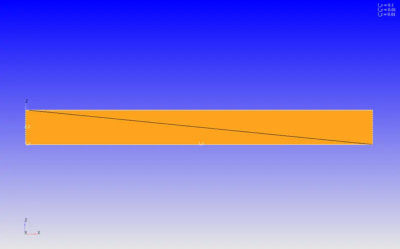
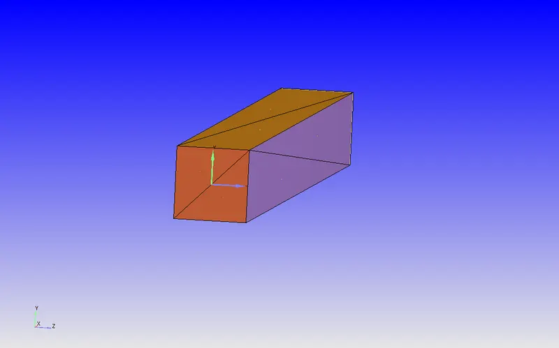
The geomertry is considered to be a simple duct with dimensions - 0.1m*0.01m*0.01m.

3.2 Mesh

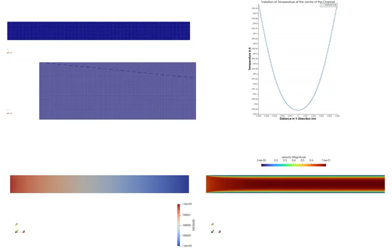
Mesh images and details wrt all the different cases are shown in the 1st image in post processing section.

4. Solver:

For all the 3 cases, the solver used is PISO, density-based.

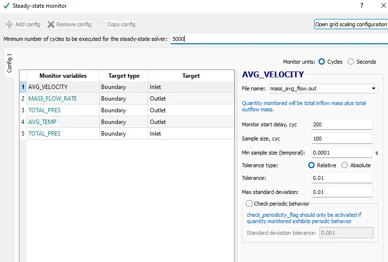
The above image indicates the steady state solver set up.
Sample size is the number of cycles for which the output values will be recorded. For this study, it is considered to be 100.
Minimum number of cycles to run is set to 5000. This means, even if the solution reaches convergence before 5000 cycles, the simulation wil still run for a minimum of 5000 cycles.

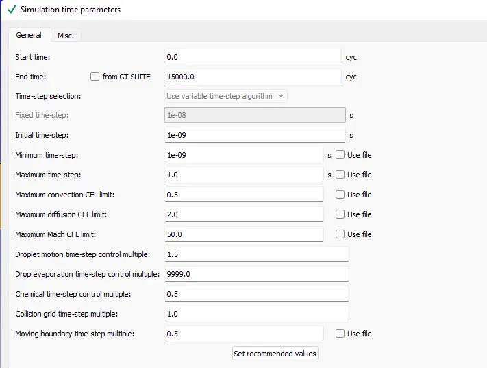
The above image indicates time parameter details for the simulations. This is kept constant for all 3 cases.

5.Post-processing:

5.1 Mesh size - 2e-4m

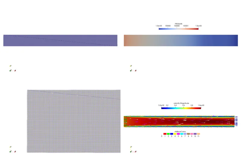
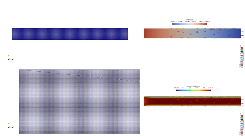
In the above image, the left portion indicates the mesh (2e-4m) and in the right portion, the top is pressure contour and the bottom is velocity contour.
In can be clearly observed that, velocity reaches a constant value after passing a certain length of the duct. This length is similar to hydrodynamic entry length.
Initially, the shear stress at the walls is maximum which decreases the velocity at the walls. Eventually, as the flow propagates, shear stress reduces and velocity becomes constant for the rest of the flow.
At this point, the flow can be termed as a fully developed flow.
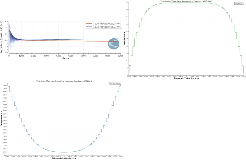
This trend can be seen for all the 3 cases considered here.
Decreasing the mesh size has resulted in increased refineness of the entry length. In these cases, the entry length is observed to reduce with decreasing the mesh size.

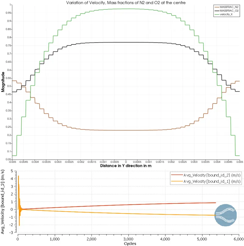
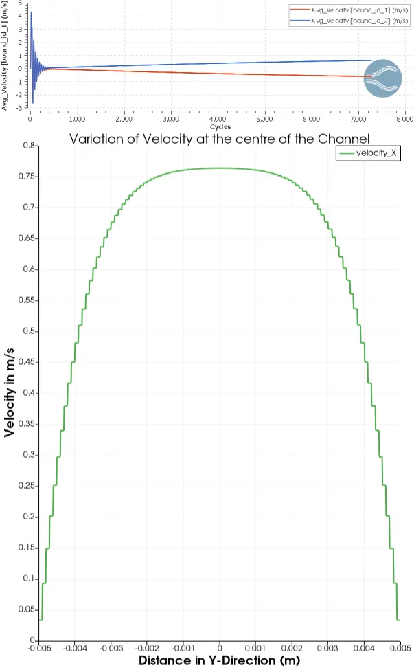
The top image indicates the variation of velocity at the mid section of channel. Since the length of channel is not large, flow will reach the fully developed status for a small length. So, at the centre of channel, flow will be fully developed.
Here, velocity is varying parabolically. Due to no-slip boundary condition, the velocity at the walls is zero and it increases and peaks at the centre. This increase is to maintain the principle of conservation of mass.
The bottom image confirms the trend observed in the top image.

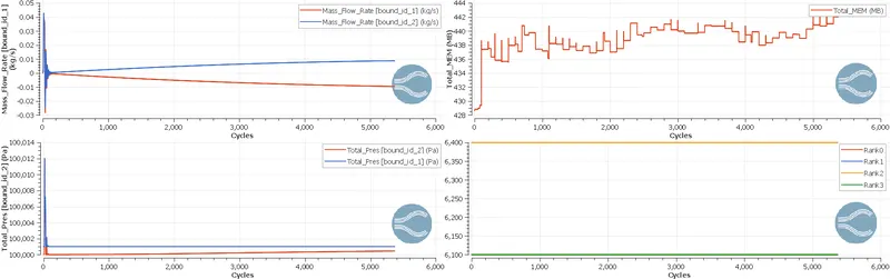
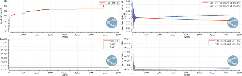
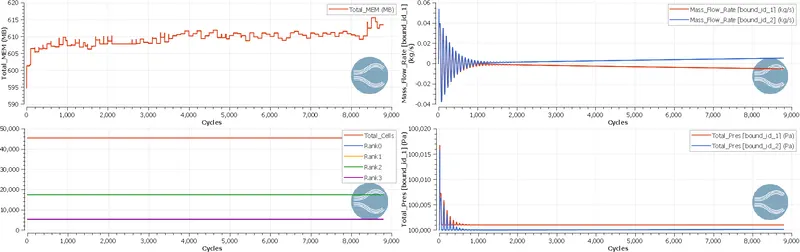
In the left portion of the above image, the top image indicates the conservation of mass at outlet and inlet. The bottom image indicates the pressure at both outlet and inlet.
The right portion of images indicates the totary memory used for simulation and the number of cells assigned for each processor.(In this study, the simulation is run parallely with 4 processors for all cases)
The results explained for this case is similar to the results in the below 2 cases. There are differences such as memory usage and variation in number of cells assigned for processors. This is due to decreased values of mesh size.
Simulation video for mesh size of 2e-4m

5.2 Mesh size - 1.5e-4