Simulation of Flow through a pipe in OpenFoam
Aim: To simulate laminar flow through a pipe using openfoam.
Problem Description:
The flow inside a circular pipe induces power losses due to frictional losses arising from the viscosity of the fluid. The losses are also caused by velocity, surface roughness of the pipe, etc. In order to minimize these losses, one needs to understand the physics of such a flow. And as this is internal flow, it is commonly observed in heating and cooling systems, combustion engines, oil pipes, water pipes, etc. These applications state the wide use of internal flow and the need to understand the nature of fluid flow.
The pipe is axis-symmetric, so only a wedge of the pipe can be considered and the results can extrapolated for the whole pipe. Here the focus is on the verfication of (Hagen-poiseullie' equations) hydrodynamic entry length, fully developed velocity profile, maximum velocity and pressure drop for fully developed flow and wall shear stress with the analytical values. Openfoam is utilized to solve this problem.
Assumptions made:
- The flow is incompressible.
- Flow is laminar.
- Pipe surface roughness has negligable effects.
- Pipe is axis-symmetric.
- Horizontal flow.
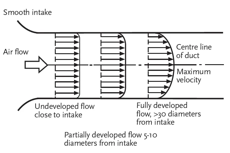
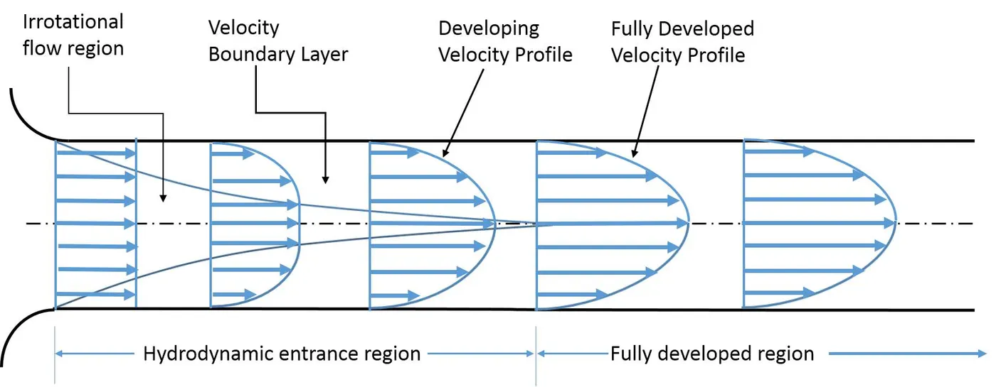
The above figures represent fluid flow inside a smooth circular pipe. At the inlet, the fluid flow is laminar and smooth and due to the viscosity of fluid(here, water), the base layers of the fluid stick to wall surface. This results in zero velocity on the pipe surface. This is called No-slip boundary condition. To maintain the momentum transfer of fluid flow, velocity increases near the centre of pipe. At a particular length of pipe(hydrodynamic entry length), the boundary layers of top and bottom surfaces merge and the fluid velocity reaches its maximum and becomes constant along with the wall shear stress. Pressure varies linearly along 'z' direction. From this point onwards, the fluid is termed as fully developed flow.
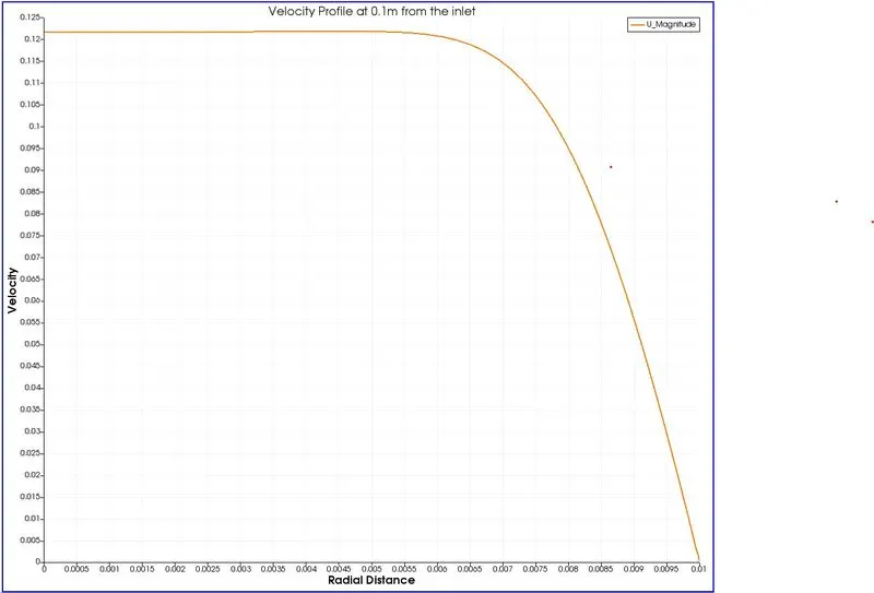
- The velocity profile is parabolic in nature and varies in the radial direction.
- For laminar flow, the hydrodynamic entrance length is: `L_e = 0.05*R_e/D`, where Re is the Reynolds number and D is the diameter of the pipe.
The cross section of the fluid is constant, circular and the flow is laminar - all these conditions apply for the use of Hagen-Poiuseiulle's equation. This equation describes the head loss across a circular cross-section pipe. The equation is given by:
`h_f = (128muQL)/(pi*rho*D^4)`, Where Q is discharge through the pipe and `mu`is the dynamic viscosity.
Shear stress is directly proportional to the velocity gradient and hence after the flow develops is decreases with velocity gradient and becomes constant.
Some assumptions are made wrt the dimensions of the cylinder and mesh generation and they are:
- Diameter = 0.02m.
- Pipe length = 2.5m
- Reynolds number = 2100.
- Number of divisions in x direction = 50.
- Number of divisions in y direction = 1.
- Number of division in z direction = 200.
- Cell expansion ratio in x direction = 0.1.
- Density of water at 298k = 997kg/m^3.
- Dynamic viscosity of water at 298k = 0.00089 Pa.s.
- Wedge angle = `3^circ`.
Governing Equations: The Navier-Stokes equations governing incompressible, laminar and viscous flow are (in cylindrical co-ordinates)
- Momentum equation: `(delv_z)/(delt) + v_r*(delv_z)/(delr)+(1/r)*v__theta*(delv_z)/(deltheta) + v_z * (delv_z)/(delz) = -1/rho * (delp)/(delz) + mu/rho*[1/r * del/(delr)(r * (delv_z)/(delr)) + 1/r^2*(del^2v_z)/(deltheta^2) + (del^2v_z)/(delz^2))]`
- The above equation is reduced to `mu/r*d/(dr)(r*(dv_z)/(dr)) = (dp)/(dz)`
- As the pressure is function of pipe length (z), the term `(dp)/(dz)`is a constant.
- Continuity equation: `1/r*del/(delr)(r*v_r) + 1/r*(delv_theta)/(deltheta) + (delv_z)/(delz) = 0`
- Velocity varies only along the radial direction and hence it is a function of Pipe radius.
Calculations:
Below are the formuale used for calculations:
%Calculations
Le = 0.05 * Re * D; %Hydrodynamic Entry Length.
V_avg = (Re * mu)/(rho * D); %Average Velocity.
V_max = 2 * V_avg; %Maximum Velocity.
delta_P = (8 * mu * L * V_avg)/(R^2); %Pressure loss.
tau = (delta_P * D)/(4 * L); %Wall Shear Stress.
Results:
- Le = 2.1m.
- V_avg = 0.0937 m/s.
- V_max = 0.1875 m/s.
- delta_P = 16.68 Pa.
- tau = 0.0334 Pa.
Geometry and Mesh description:
The pipe is assumed to be axis-symmetric, hence a wedge of the pipe can be selected and results will be the same and simulation time will be lower. In this simulation the wedge angle selected is `3^circ`.
As the image below indicates 2 wedges are created -front and back, by collapsing certain vertices. This can be seen in blockMeshDict code attached below. Collapsing of vertices is important to get the wedge shape.
blockMeshDict file:
/*--------------------------------*- C++ -*----------------------------------*
  =========                 |
        /  F ield         | OpenFOAM: The Open Source CFD Toolbox
       /   O peration     | Website:  https://openfoam.org
      /    A nd           | Version:  8
     /     M anipulation  |
*---------------------------------------------------------------------------*/
FoamFile
{
    version     2.0;
    format      ascii;
    class       dictionary;
    object      blockMeshDict;
}
// * * * * * * * * * * * * * * * * * * * * * * * * * * * * * * * * * * * * * //

convertToMeters 1;

vertices
(
    (0.00000000 0.00000000 0.00000000)
    (0.00000000 0.00999657 -0.00026177)
    (0.00000000 0.00999657 0.00026177)
    (2.50000000 0.00000000 0.00000000)
    (2.50000000 0.00999657 -0.00026177)
    (2.50000000 0.00999657 0.00026177)
);

blocks
(
    hex (0 1 2 0 3 4 5 3) (50 1 200) simpleGrading (0.100000 1.000000 1.000000)
);

edges
(
    arc 1 2 (0 0.010000 0)
    arc 4 5 (2.500000 0.010000 0)
);

boundary
(
    axis
    {
        type empty;
        faces
        (
            (0 3 3 0)
        );
    }

    inlet
    {
        type patch;
        faces
        (
            (0 2 1 0)
        );
    }

    wall
    {
        type wall;
       faces
        (
            (2 5 4 1)
        );
    }

    outlet
    {
        type patch;
        faces
        (
            (3 4 5 3)
        );
    }

    front
    {
        type wedge;
        faces
        (
            (0 3 5 2)
        );
    }

    back
    {
        type wedge;
        faces
        (
            (0 1 4 3)
        );
    }
);

mergePatchPairs
(
);

// ************************************************************************* //
The above file was generated through a Matlab code which is provided in the subsequent section. Below are some of the mesh images.
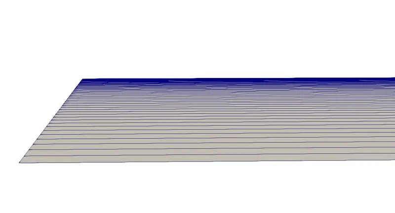
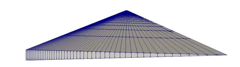

Cell expansion ratio is the ratio of width of end cell on an edge to the starting cell of the same edge. By using specific cell expansion ratios, the mesh can be refined near regions of importance. In this case 0.1 is used near the wall, as it is the region of importance.
Boundary and Initial conditions:
Pressure
/*--------------------------------*- C++ -*----------------------------------*
  =========                 |
        /  F ield         | OpenFOAM: The Open Source CFD Toolbox
       /   O peration     | Website:  https://openfoam.org
      /    A nd           | Version:  8
     /     M anipulation  |
*---------------------------------------------------------------------------*/
FoamFile
{
    version     2.0;
    format      ascii;
    class       volScalarField;
    object      p;
}
// * * * * * * * * * * * * * * * * * * * * * * * * * * * * * * * * * * * * * //

dimensions      [0 2 -2 0 0 0 0];

internalField   uniform 0;

boundaryField
{
    axis
    {
        type		empty;
    }

    inlet
    {
        type		zeroGradient;
    }

    wall
    {
        type		zeroGradient;
    }

    outlet
    {
        type		fixedValue;
        value		uniform 0.01669;
    }

    front
    {
        type		wedge;
    }

    back
    {
        type		wedge;
    }
}

// ************************************************************************* //
Velocity:
/*--------------------------------*- C++ -*----------------------------------*
  =========                 |
        /  F ield         | OpenFOAM: The Open Source CFD Toolbox
       /   O peration     | Website:  https://openfoam.org
      /    A nd           | Version:  8
     /     M anipulation  |
*---------------------------------------------------------------------------*/
FoamFile
{
    version     2.0;
    format      ascii;
    class       volVectorField;
    object      U;
}
// * * * * * * * * * * * * * * * * * * * * * * * * * * * * * * * * * * * * * //

dimensions      [0 1 -1 0 0 0 0];

internalField   uniform (0.09361 0 0);

boundaryField
{
    axis
    {
        type		empty;
    }

    inlet
    {
        type		fixedValue;
        value		uniform (0.09361 0 0);
    }

    wall
    {
        type		fixedValue;
        value		uniform (0 0 0);
    }

    outlet
    {
        type		zeroGradient;
    }

    front
    {
        type		wedge;
    }

    back
    {
        type		wedge;
    }

}

// ************************************************************************* //
Physical Properties:
/*--------------------------------*- C++ -*----------------------------------*
  =========                 |
        /  F ield         | OpenFOAM: The Open Source CFD Toolbox
       /   O peration     | Website:  https://openfoam.org
      /    A nd           | Version:  8
     /     M anipulation  |
*---------------------------------------------------------------------------*/
FoamFile
{
    version     2.0;
    format      ascii;
    class       dictionary;
    location    "constant";
    object      transportProperties;
}
// * * * * * * * * * * * * * * * * * * * * * * * * * * * * * * * * * * * * * //

nu              [0 2 -1 0 0 0 0] 8.8891e-7;


// ************************************************************************* //
controlDict file:
/*--------------------------------*- C++ -*----------------------------------*
  =========                 |
        /  F ield         | OpenFOAM: The Open Source CFD Toolbox
       /   O peration     | Website:  https://openfoam.org
      /    A nd           | Version:  8
     /     M anipulation  |
*---------------------------------------------------------------------------*/
FoamFile
{
    version     2.0;
    format      ascii;
    class       dictionary;
    location    "system";
    object      controlDict;
}
// * * * * * * * * * * * * * * * * * * * * * * * * * * * * * * * * * * * * * //

application     icoFoam;

startFrom       startTime;

startTime       0;

stopAt          endTime;

endTime         27;

deltaT          0.005;

writeControl    timeStep;

writeInterval   20;

purgeWrite      0;

writeFormat     ascii;

writePrecision  6;

writeCompression off;

timeFormat      general;

timePrecision   6;

runTimeModifiable true;


// ************************************************************************* //
Matlab code used to automate blockMeshDict file generation:
clear all
close all
clc

%Inputs
D = input('Enter pipe Diameter:'); %Diameter of the pipe is assumed to be 0.035m for this case.
R = D/2; %Radius
L = input('Enter pipe Length:'); %Total pipe length is assumed to be 5m.
Re = input('Enter Reynolds number:'); %Reynolds number considerd is 2100.
nx = input('Enter the number of divisions in x direction:');
ny = input('Enter the number of divisions in y direction:');
nz = input('Enter the number of divisions in z direction:');
x = input('Enter Cell Expansion ratio in x direction:');
y = input('Enter Cell Expansion ratio in y direction:');
z = input('Enter Cell Expansion ratio in z direction:');
rho = 997; %Density of water at 298k.
mu = 8.9*10^-4; %Dynamic viscosity of water at 298k.


theta = input('Enter wedge angle: ');

%Calculations
Le = 0.05 * Re * D; %Hydrodynamic Entry Length.
V_avg = (Re * mu)/(rho * D); %Average Velocity.
V_max = 2 * V_avg; %Maximum Velocity.
delta_P = (8 * mu * L * V_avg)/(R^2); %Pressure loss.
tau = (delta_P * D)/(4 * L); %Wall Shear Stress.

%Vertices of the wedge
v1 = [0 0 0]; %Vertex #1.
v2 = [0 (R*cosd(theta/2)) -(R*sind(theta/2))]; %Vertex #2.
v3 = [0 (R*cosd(theta/2)) (R*sind(theta/2))]; %Vertex #3.
v4 = [L 0 0]; %Vertex #4.
v5 = [L (R*cosd(theta/2)) -(R*sind(theta/2))]; %Vertex #5.
v6 = [L (R*cosd(theta/2)) (R*sind(theta/2))]; %Vertex #6.


h = fopen('blockMeshDict.txt','w'); %File handle.

%First few lines of the blockMeshDict file

fprintf(h,'/*--------------------------------*- C++ -*----------------------------------*n');
fprintf(h,'  =========                 |n');
fprintf(h,'        /  F ield         | OpenFOAM: The Open Source CFD Toolboxn');
fprintf(h,'       /   O peration     | Website:  https://openfoam.orgn');
fprintf(h,'      /    A nd           | Version:  8n');
fprintf(h,'     /     M anipulation  |n');
fprintf(h,'*---------------------------------------------------------------------------*/');

fprintf(h,'nFoamFilen');
fprintf(h,'{n');
fprintf(h,'    version     2.0;n');
fprintf(h,'    format      ascii;n');
fprintf(h,'    class       dictionary;n');
fprintf(h,'    object      blockMeshDict;n');
fprintf(h,'}n');
fprintf(h,'// * * * * * * * * * * * * * * * * * * * * * * * * * * * * * * * * * * * * * //n');

fprintf(h,'nconvertToMeters 1;n');
fprintf(h,'nverticesn(n');

%Entering Vertices

fprintf(h,'    (%0.8f %0.8f %0.8f)n',v1);
fprintf(h,'    (%0.8f %0.8f %0.8f)n',v2);
fprintf(h,'    (%0.8f %0.8f %0.8f)n',v3);
fprintf(h,'    (%0.8f %0.8f %0.8f)n',v4);
fprintf(h,'    (%0.8f %0.8f %0.8f)n',v5);
fprintf(h,'    (%0.8f %0.8f %0.8f)n);n',v6);

%Creating blocks

fprintf(h,'nblocksn(n');
fprintf(h,'    hex (0 1 2 0 3 4 5 3) (%d %d %d) simpleGrading (%f %f %f)n);n',nx,ny,nz,x,y,z); %Hexahedral block.

%Creating edges

fprintf(h,'nedgesn(n');
fprintf(h,'    arc 1 2 (0 %f 0)n    arc 4 5 (%f %f 0)n);n',R,L,R); %Front and Rear arcs.

%Creating boundaries

fprintf(h,'nboundaryn(n    axisn    {n');
fprintf(h,'        type empty;n        facesn        (n            (0 3 3 0)n        );n    }n'); %Axis.
fprintf(h,'n    inletn    {    n        type patch;n        facesn        (n            (0 2 1 0)n        );n    }n'); %Inlet.
fprintf(h,'n    walln    {    n        type wall;n       facesn        (n            (2 5 4 1)n        );n    }n'); %Wall.
fprintf(h,'n    outletn    {    n        type patch;n        facesn        (n            (3 4 5 3)n        );n    }n'); %Outlet.
fprintf(h,'n    frontn    {    n        type wedge;n        facesn        (n            (0 3 5 2)n        );n    }n'); %Front.
fprintf(h,'n    backn    {    n        type wedge;n        facesn        (n            (0 1 4 3)n        );n    }n);n'); %Back.

%Merging all the patches

fprintf(h,'nmergePatchPairsn(n);n');
fprintf(h,'n// ************************************************************************* //n');
Post-processing: Results
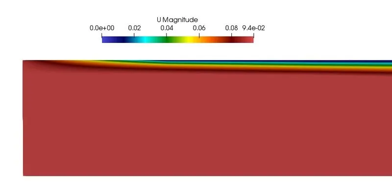
Velocity at the inlet of the pipe (m/s)
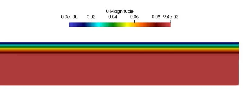
Velocity at the pipe outlet (m/s)
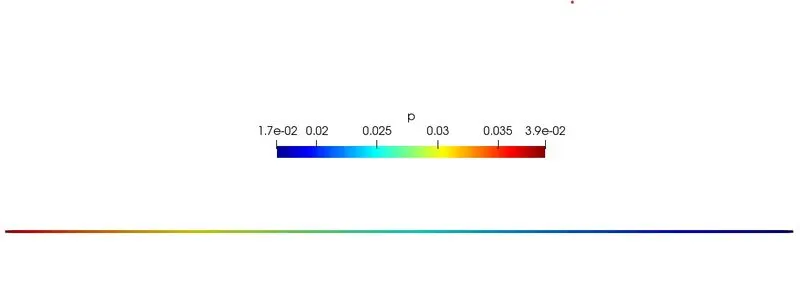
Pressure field in circular pipe (`m^2/s^2`)
- It can be seen from the above graph, that the velocity profile at the inlet is still developing and the viscous effects are just beginning to affect the flow.
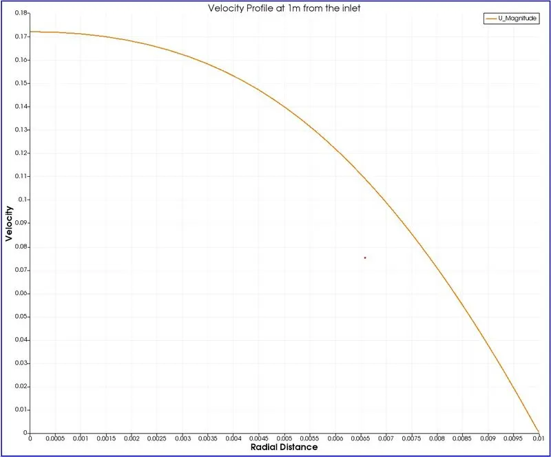
- At 1m from the inlet, viscous effects have increased and the velocity is reaching its maximum value at the centre of pipe.
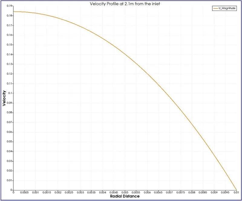
- 2.1 m is the anlytical value of hydrodynamic entry length and the above graph indicates, at 2.1m from the inlet, the velocity of the fluid to be 0.1842m/s whereas the analytical result is 0.1872m/s . The error between analytical and simulation result is 1.6%, which is acceptable.
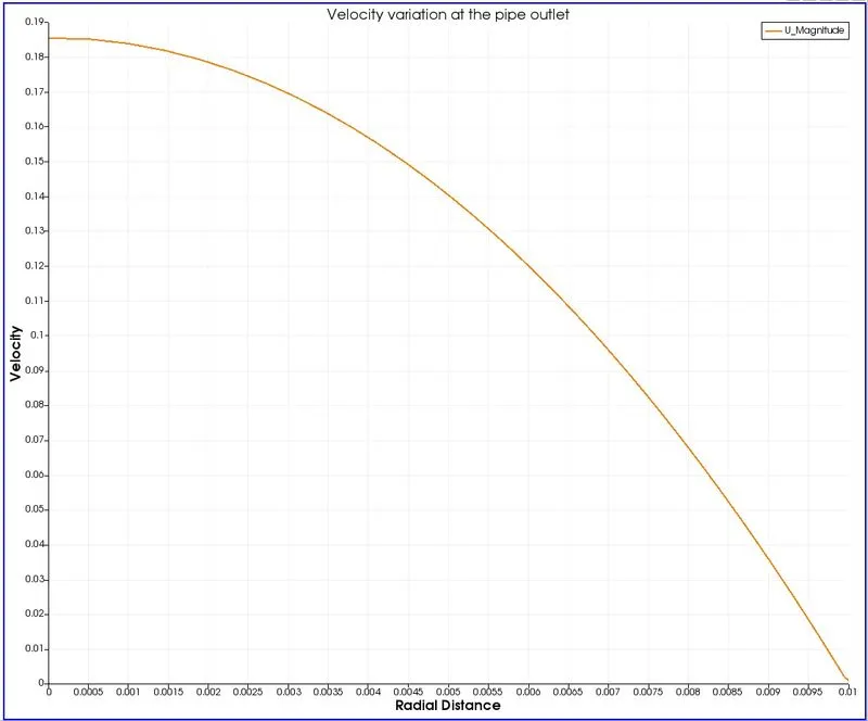
- At the outlet, the flow has been fully developed and the maximum velocity is the same as at the hydrodynamic entrance length.
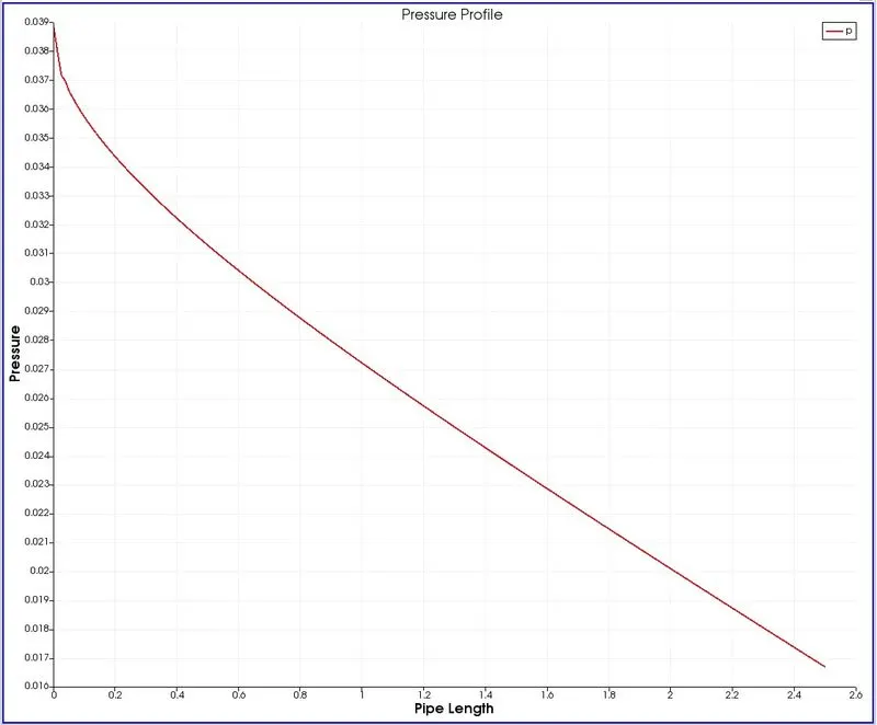
- The above graph indicates pressure drop along the pipe and the simulation result is 0.01696 `m^2/s^2`and the analytical result is 0.01669 `m^2/s^2`. The error percentage is -1.61.
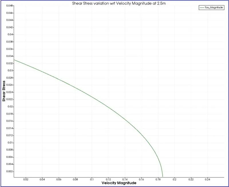
- Shear stress is directly proportional to velocity gradient. The above graph indicates variation of shear stress wrt to velocity magnitude. Shear stress is the greatest near the walls. At the inlet, viscosity of the fluid has a strong effect on velocity gradient and velocity magnitude.
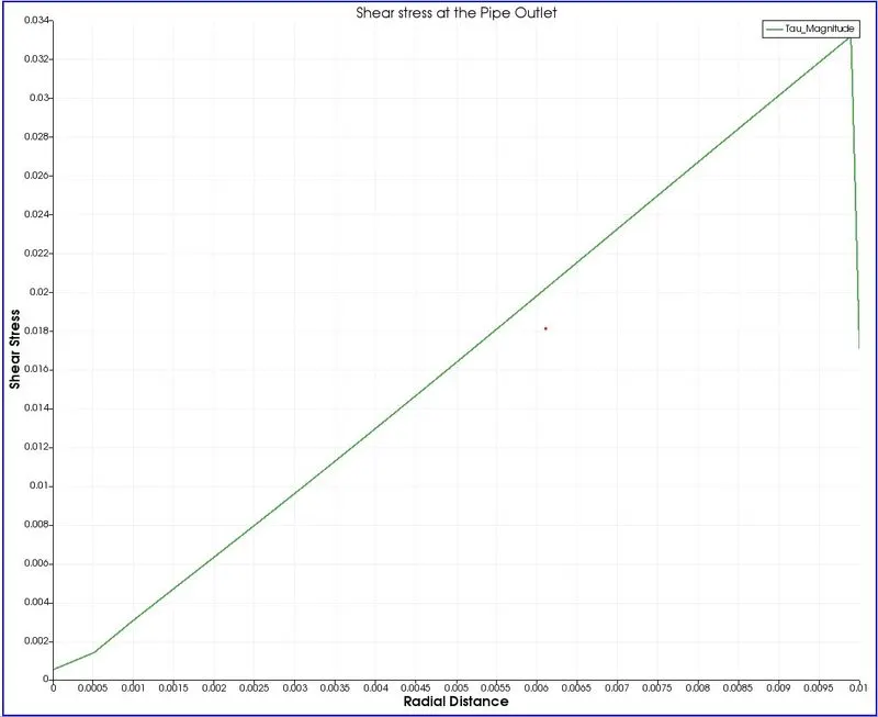
- Above graph indicates wall shear stress at pipe outlet. The simulation result is 0.03331Pa and the analytical result is 0.03328Pa. The error percentage is -0.091.
Conclusions:
- The hydrodynamic length of 2.1m is validated in the simulation result.
- Velocity profile for flow through pipe is accurately predicted and maximum velocity, pressure drop values are obtained within the standard error percentage.
- Shear stress is validated for the flow.
Below table indicates the errors between analytical and simulation results:
|
Sl.No |
Variable |
Simulation result |
Analytical result |
Error |
|
1. |
Maximum velocity |
0.1842m/s |
0.1872m/s |
+1.6% |
|
2. |
Pressure drop |
0.01696 m^2/s^2 |
0.01669 m^2/s^2 |
-1.61% |
|
3. |
Wall shear stress |
0.03331Pa |
0.03328Pa |
-0.091% |