Rayleigh-Taylor Instability
Aim: To perform Rayleigh-Taylor Simulation for -
- Mesh size 0.5mm
- Mesh size 0.1mm
- User-defined material with mesh size 0.1mm
and
- To describe some CFD models based on the mathematical analysis of Rayleigh-Taylor instability.
- To state the effects of variation in Atwood number on the behaviour of instability.
Introduction:
Rayleigh-Taylor instability is a type of hydrodynamic instability which arises due to density differences between 2 fluids that are placed one on top of the other. The fluid on top is denser than the bottom fluid. This creates an instability at the interface. If the lighter fluid maintains sufficiient pressure, then the interface will remain undisturbed.
But a slightest disturbance can cause the interface to become unstable, after which the heavier fluid moves, accelerating with gravity and lighter fluid rises as bubbles into the heavier fluid due to buoyancy forces.
For the base case simulations, water and air are considered. The major forces that contribute towards this instability are hydrodynamic pressure and the buoyancy force.
This instability along with others described below are important in various fields such as Astrophysics, Inertical Confinement fusion(ICF), Food processing, Nuclear explosions, volcanic eruptions, Plasma fusion, etc.
Theory:
Rayleigh-Taylor instability happens at the interface of two different density fluids. There are a few CFD models that are based on this instability.
- Richtmeyer-Meshkov instability
This instability also occurs at the interface of two fluids, but the cause of perturbation is shock wave. The flow equations are analyzed by understanding the velocity field where perturbations at the interface are created due to shock wave. Also, the flow, once shock wave passes is treated as incompressible, as the perturbation velocity is assumed to be much smaller than the speed of sound.
- Granular Rayleigh-Taylor instability
This instability arises when a layer of dense grains are placed above a layer of air. Initially the interface will be flat, but due to density differences granular finger like shape starts forming once the grains start to fall and these fingers are separated by rising air bubbles. This results of this instability can be quatified by means of fourier series.
- Kelvin-Helmholtz instability
This is observed where there are 2 streams of materials, each having different velocity and different density. The lower stream will be more dense. Initially at the interface a small perturbation arises, which increases eventually to become exponential. This distribution results in the formation of vortex sheet. This instability at the interface can be assumed to be sine wave and the vortex sheet present induces a rotational velocity near the undisturbed points of the sine wave causing the instability to grow and eventually break in a turbulent fashion.
Approach:
To simulate the instability, the conditions and values considered in terms of geometrical and computational aspects are mentioned below.
Geometrical aspects:
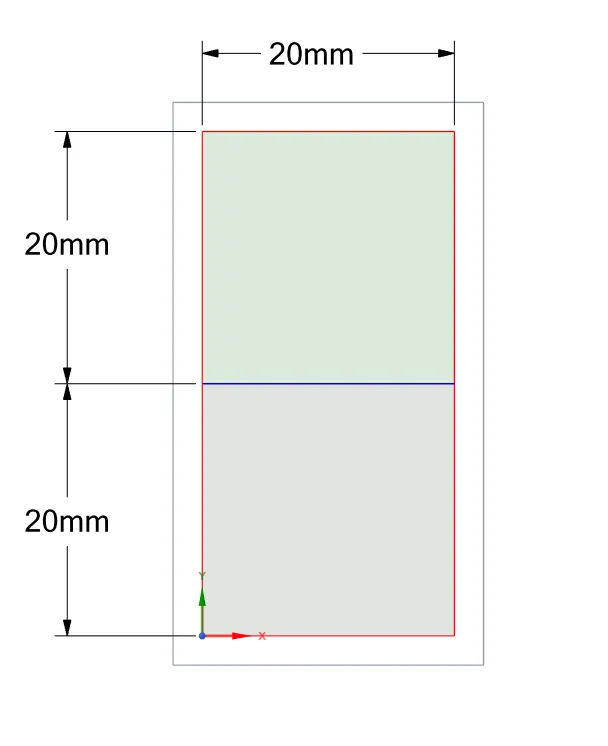
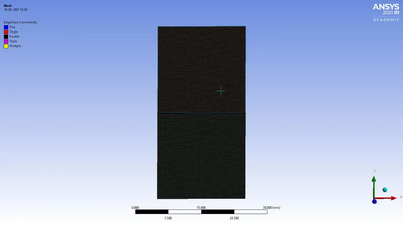
- Two square blocks of size (20*20)`cm^2`are used to build the required geometry.
- For this case, mesh size is 0.5mm and in the next case the mesh size of 0.1mm is considered to understand how does mesh refinement affect the instability.
- Number of elements - 3200, Number of nodes - 3321 for mesh size 0.5mm and for mesh size 0.1mm - Number of elements - 80000, nodes - 80601.
- Share topology option in Spaceclaim is used to connect the interface between 2 blocks.
Computational aspects:
- Pressure based solver is used.
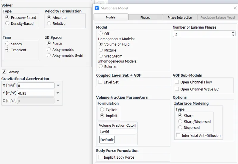
- As the problem involves simultaneous flow two fluids in different phases, Multiphase flow option is used in fluent.
- In Multiphase, implicit formulation is used.
- Transient method is employed in this study.
- For the first two cases water is used as the denser fluid and air is considered as the lifghter fluid. The flow is assumed to be laminar.
- The importance in this problem is on the interface between 2 fluids and hence a surface tracking model would accurately serve the purpose. So Volume of fluid model is used.
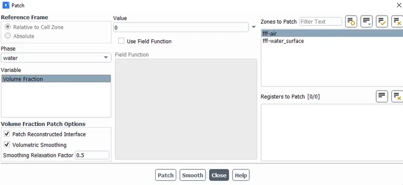
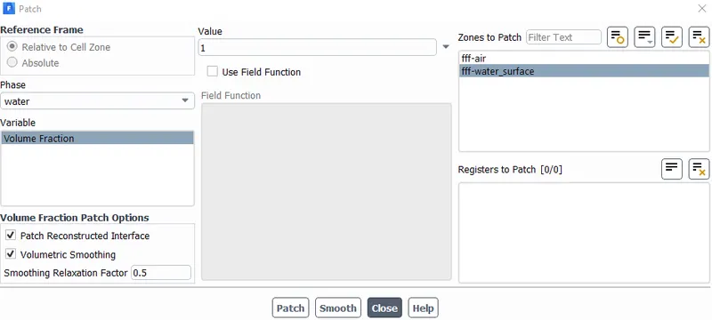
- After the problem is initialized, two different blocks are patched by volume fraction. The value is 0 for the block containing air and for the other block, it is 1.
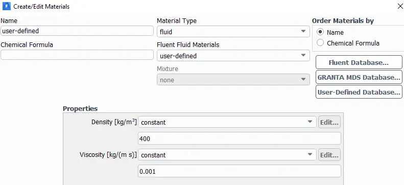
- For case 3, a user defined material is used for lighter fluid with density 400`(kg)/m^3` and viscosity 0.001`(kg)/(ms)`.
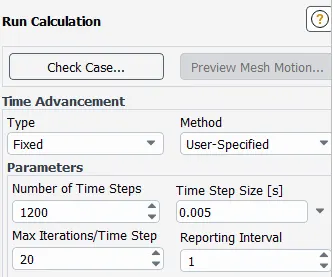
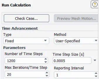
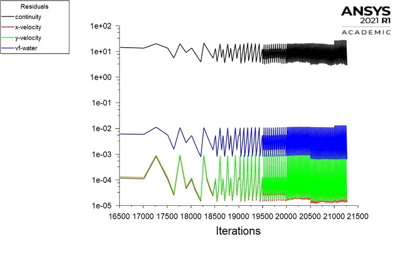
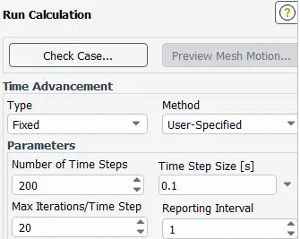
- For the first case, time step size is 0.005, for the second case time step size is 0.0005 and for the last case time step size is 0.1.
- For the first two cases number of time steps is 1200 and for the last case, it is 200.
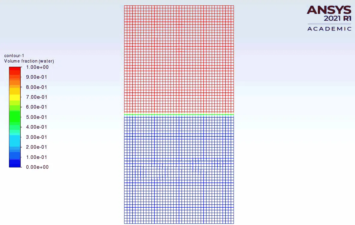
1. Simulation results for base mesh size of 0.5mm:
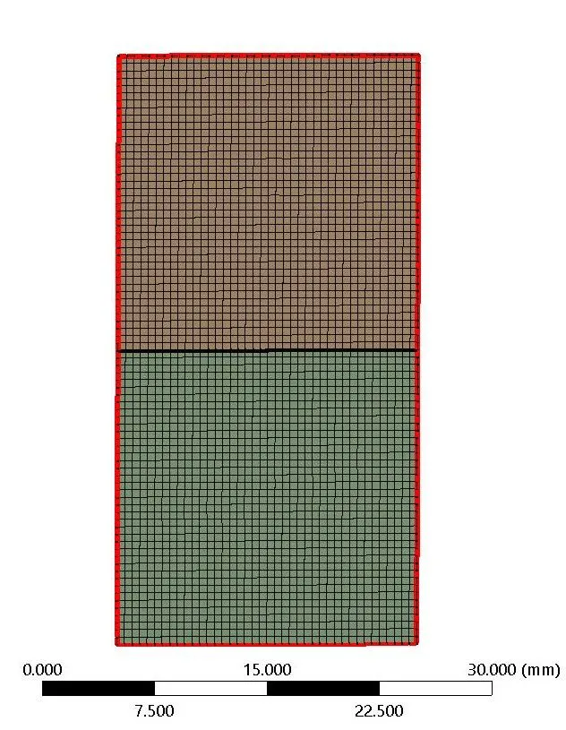
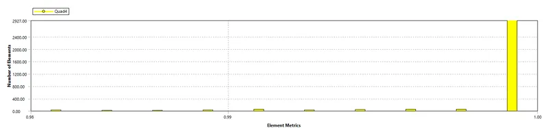
Mesh Quality:
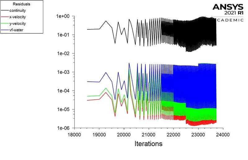
Calculation details:
Results:
 - Fig1
 - 2
- 2
2. Simulation results for mesh size of 0.1mm:
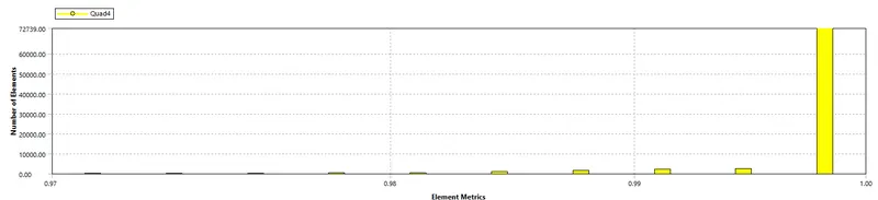
Mesh quality:
Calculation details:
Results:
 - Fig3
 - 4
- 4
How do simulations of case1 and case2 differ?
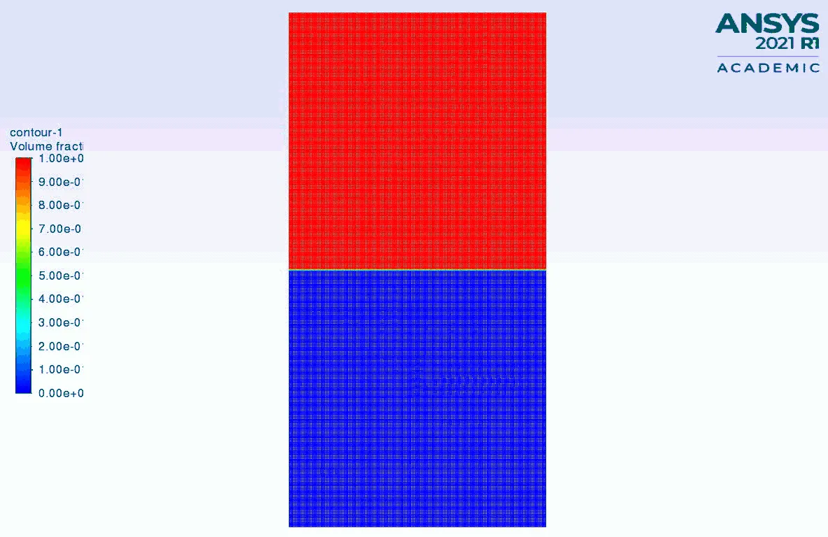
2 and 4 represent the animations for mesh sizes 0.5mm and 0.1mm respectively. The time step size used in case 2 is lower than case 1. This is because in case 2 for the time step size of 0.005, floating point error was observed. So to avoid this, time step size has been decreased to 0.0005.
It can also be observed that the details in the animation is more in case 2 because of refined mesh. This is an advantage along with accuracy. But the computational time is high for case 2 due to refined mesh and lower time step size. If the purpose of the simulation is just to observe the simple flow behaviour, then first case is enough. But if more accuracy is necessary as to how small changes in time affect specific places in the flow field, then case 2 is better suited.
Why transient? and Why not steady?
Flow field behaves differently with time in these kind of problems. That is, with time, there is no uniform change within the flow field. If steady method is used, then it won't be able to capture the detailed instabilities (it just focuses on the end result, while here observing the time dependent flow behaviour is important), which is the major focus of this study.
As this is a developing flow, using transient method is the best way to observe the instability effects.
3. Simulation results for user defined material with refined mesh (0.1mm):
User defined material:
Calculation details:
Results:
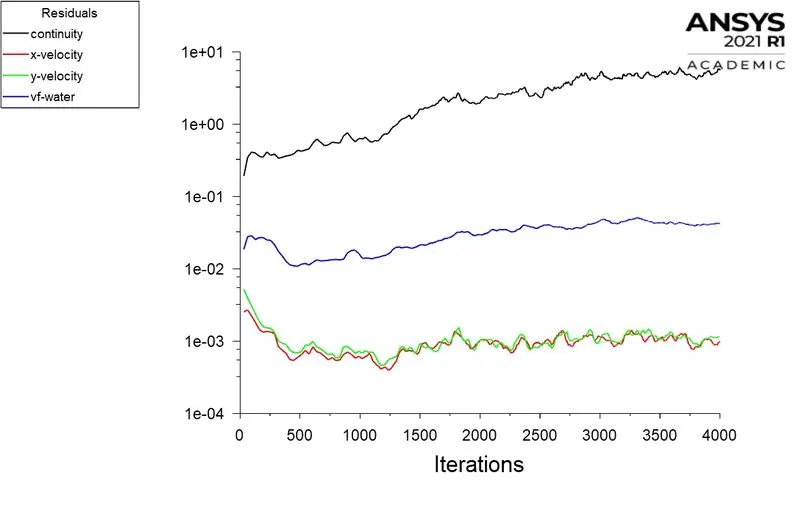 - Fig5
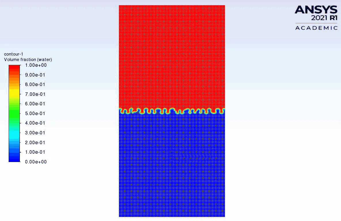 - 6
- 6
How does Atwood number affect the behaviour of instability?
Atwood number is a dimensionless number given by `A = (rho_2-rho_1)/(rho_2+rho_1)`.
Calculation for case A: Water and air
`A = (1000-1.225)/(1000+1.225) = 0.9975.`
- For the first case, the Atwood number is close to 1. For such cases, lighter fluid below rises as bubbles. Among these bubbles, ones having higher velocity move upwards and may combine with neighbouring bubbles to get larger and on the other hand, lower size bubbles shrink further and move downwards.
- The bubbles at the bottom eventually move upwards due to hydrodynamic pressure and combine with the top layer. This can be observed in the above cases 1 and 2.
- It can also be seen that the settling rate is higher in this case. This is becaue of the increased growth rates of bubbles which is due to higher Atwood number.
Calculation for case B: User defined material and Water
`A = (1000-400)/(1000+400) = 0.4285.`
- Decrease in Atwood number casues decrease in growth rates and rate of acceleration of heavier fluid. Logically this is due to the increased density of lower fluid, with almost the same viscosity as the top fluid.
- In the beginning of the animation, small finger like structures can be observed which accelerate with time. But the growth rate decreases from being exponential in the beginning to lower values proportional to Atwood number.
- In case 3, the above conclusions can be observed. It takes more time to settle for the such cases due to the low density differences.
References: