Auto ignition using Cantera
Aim:To simulate Auto-ignition time for methane using Cantera for different conditions mentioned below -
- Variation of Auto Ignition time of Methane with a constant temperature of 1250K and pressure varying from 1 to 5 atm
- Variation of Auto Ignition time of Methane with a constant pressure of 5 atm and temperature varying from 950K to 1450K
- Variation of molar concentration of elements - H2O, O2 and OH wrt igniton time
1. Introduction:
The lowest temperature at which ignition starts is the Auto-ignition temperature. This temperature can vary based on the initial temperature, pressure and element concentrations. There is also time associated with autoignition which is called Ignition delay. Once the fuel and air mixture are together, after certain time the ignition begins and this time gap is referred to as ignition delay. Fuels are characterized by ignition delay.
Lower the initial temperature, higher will be the ignition delay. But this is not always true. There is a term called Negative temperature co-efficient regime, which indicates the region on the ignition time vs temperature. In this region, as the initial or ignition temperature increases, the ignition delay increases for some time before dipping. This is also a property of fuels, which means that it varies for different fuels.
Practically there are experiments utilized to estimate ignition delay such as - the shocktube experiment and rapid combusiton experiment. In terms of equations, to determine ignition delay, only species and energy equations has to be solved - through these equations rate of temperature rise can be calculated. So, when ignition starts, the temperature hikes very rapidly and attains the maximum value. Through this value, ignition delay can be calculated.
To satisfy the current aims, Cantera is used. In Cantera, different reactors can be used based on the problem requirement. Each reactor will have certain volume and its own governing equations. The details of governing equations are provided in the Cantera website. In a reactor, at a particular state, properties such as temperature and pressure remain constant.
Based on the reactor defined, a reactor network can be used, which integrates all different states of the reactor using advance method. The simulation presented here is the 0D simulation, as only temporal evolution of the gas mixture towards equilibrium is considered.
2. Coding approach:
- All the necessary libraries are imported.
- A gas instance is created from Solution class - in this case it's Methane.
- Temperature, Pressurea and Molar concentrations are defined.
- A suitable reactor is selected and is filled with the gas considered for simulation.
- A reactor network is created to integrate all the states of the reactor.
- An instance called states is created which containes solutions of all parameters at all states.
- A for loop is created to advance the reactor and integrate it from one state to another. Simulation time considered is 10seconds.
- The program is made to integrate for a total of 1mili second at once.
- After advancing the reactor, the solution is stored in the solution array.
- All of the above steps are combined to write a function with input temperature, pressure and molar concentration of species.
- Variation of Temperature, pressure and Molar concentration is plotted against ignition time.
- To calculate ignition delay, maximum temperature is used.
3. Code:
3.1 Variation of molar concentration of elements - H2O, O2 and OH wrt igniton time - Code
def cv_combustion(T, P, species_concentration):

	#import sys
	import cantera as ct
	import numpy as py
	import matplotlib.pyplot as plt

	methane = ct.Solution('gri30.xml')
	methane.TPX = T, P, species_concentration
	reactor = ct.IdealGasReactor(methane)

	reactor_network = ct.ReactorNet([reactor])

	states = ct.SolutionArray(methane,extra=['time_in_ms','t'])
	time = 0.0
	mol_frac = py.zeros((10000,3))

	for a in range(10000):
		time += 1e-3
		reactor_network.advance(time)
		states.append(reactor.thermo.state, time_in_ms = time*1e3, t = time)
		mol_frac[a,:] = reactor.thermo['H2O','O2','OH'].X

	return (states, mol_frac)


import matplotlib.pyplot as plt

#For change of molar concentrations
[states1, mol_frac1] = cv_combustion(1000, 5*101325, {'CH4':1, 'O2':2, 'N2':7.52})

plt.figure()
plt.plot(states1.t, mol_frac1[:,0])
plt.xlabel('Time in seconds')
plt.ylabel('Molar Concentration of H2O')
plt.title('Variation of Molar Concentration of Species wrt Timen' 'for Temperature = 1000k and Pressure = 5bar')

plt.figure()
plt.plot(states1.t, mol_frac1[:,1])
plt.xlabel('Time in seconds')
plt.ylabel('Molar Concentration of O2')
plt.title('Variation of Molar Concentration of Species wrt Timen' 'for Temperature = 1000k and Pressure = 5bar')

plt.figure()
plt.plot(states1.t, mol_frac1[:,2])
plt.xlabel('Time in seconds')
plt.ylabel('Molar Concentration of OH')
plt.title('Variation of Molar Concentration of Species wrt Timen' 'for Temperature = 1000k and Pressure = 5bar')
plt.show()


[states2, mol_frac2] = cv_combustion(500, 5*101325, {'CH4':1, 'O2':2, 'N2':7.52})

plt.figure()
plt.plot(states2.t, mol_frac2[:,0])
plt.xlabel('Time in seconds')
plt.ylabel('Molar Concentration of H2O')
plt.title('Variation of Molar Concentration of Species wrt Timen' 'for Temperature = 500k and Pressure = 5bar')

plt.figure()
plt.plot(states2.t, mol_frac2[:,1])
plt.xlabel('Time in seconds')
plt.ylabel('Molar Concentration of O2')
plt.title('Variation of Molar Concentration of Species wrt Timen' 'for Temperature = 500k and Pressure = 5bar')

plt.figure()
plt.plot(states2.t, mol_frac2[:,2])
plt.xlabel('Time in seconds')
plt.ylabel('Molar Concentration of OH')
plt.title('Variation of Molar Concentration of Species wrt Timen' 'for Temperature = 500k and Pressure = 5bar')
plt.show()
3.11 Results
3.11.1 For temperature of 500k and pressure of 5bar
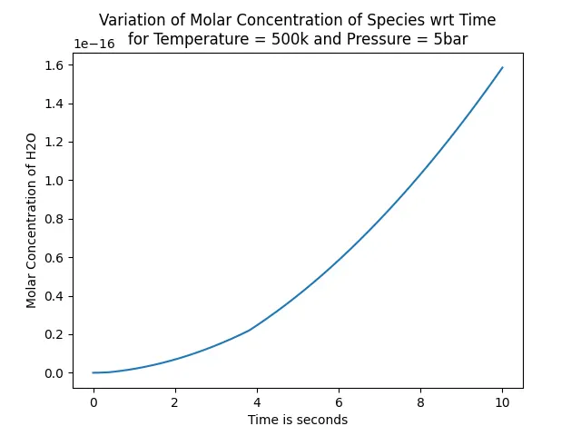
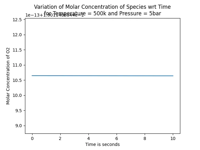
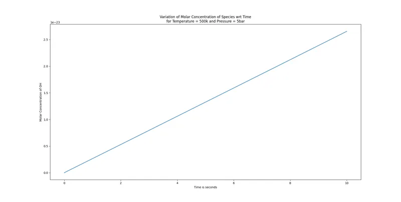
- Reduced temperature slows down the reaction rate. This can be seen in the above images.
- The ignition temperature of Methane is `537^0C`. For this case, the initial temperature given is 500k which is very less. So the rate of formation of products and the rate of combustion of reactants is less.
- Due to low initial temperature, time taken to reach ignition temperature is less and formation of products such OH and H2O is less as can be seen in the images.
- On the reactant side, O2 is consumed in very less quantities, so the concentration of products, although they are being formed, is lower. This is why O2 appears constant throughout the simulation time of 10 seconds.
3.11.2 For temperature of 1000k and pressure of 5bar
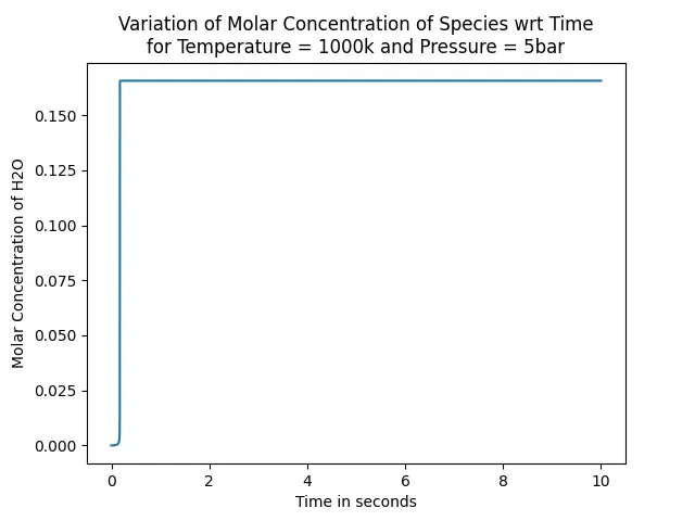
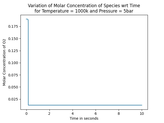
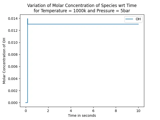
- Increasing either pressure or temperature of a system increases the rate of reaction and that is results with this case. The pressure is 5bar and temperature is 1000k.
- It can be seen that apart from the reactant O2, the products H2O and OH rise in concentration exponentially at ignition start time. These elements reach their maxiumum concentration values at this time and this can be used to calculate autoignition time.
- After this time, the concentration remains constant.
- And for O2, since its a reactant it concentration drops exponentially at iginition start time due to rapid combustion.
- In this case, pressure and temperature are both optimal for the reaction to proceed at a normal rate.
3.2 Variation of Auto Ignition time of Methane with a constant pressure of 5 atm and temperature varying from 950K to 1450K - code:
def cv_combustion(T, P, species_concentration):

	import sys
	import cantera as ct
	import numpy as py
	import matplotlib.pyplot as plt

	methane = ct.Solution('gri30.xml')

	methane.TPX = T, P, species_concentration

	reactor = ct.IdealGasReactor(methane)

	reactor_network = ct.ReactorNet([reactor])

	states = ct.SolutionArray(methane,extra=['time_in_ms','t'])
	time = 0.0

	for a in range(10000):
		time += 1e-3
		reactor_network.advance(time)
		states.append(reactor.thermo.state, time_in_ms = time*1e3, t = time)

	return states

import cantera as ct
import matplotlib.pyplot as plt

atm = ct.one_atm

ignition_delays = []
Temperatures = [950, 1100, 1250, 1350, 1450]

#For different temperatures
states1 = cv_combustion(950, 5*101325, {'CH4':1, 'O2':2, 'N2':7.52})
tmax1 = states1.T.argmax()
delay_time1 = states1.t[tmax1]
ignition_delays.append(delay_time1)

states2 = cv_combustion(1100, 5*101325, {'CH4':1, 'O2':2, 'N2':7.52})
tmax2 = states2.T.argmax()
delay_time2 = states2.t[tmax2]
ignition_delays.append(delay_time2)

states3 = cv_combustion(1250, 5*101325, {'CH4':1, 'O2':2, 'N2':7.52})
tmax3 = states3.T.argmax()
delay_time3 = states3.t[tmax3]
ignition_delays.append(delay_time3)

states4 = cv_combustion(1350, 5*101325, {'CH4':1, 'O2':2, 'N2':7.52})
tmax4 = states4.T.argmax()
delay_time4 = states4.t[tmax4]
ignition_delays.append(delay_time4)

states5 = cv_combustion(1450, 5*101325, {'CH4':1, 'O2':2, 'N2':7.52})
tmax5 = states5.T.argmax()
delay_time5 = states5.t[tmax5]
ignition_delays.append(delay_time5)

plt.figure()
plt.plot(states1.t, states1.T)
plt.plot(states2.t, states2.T)
plt.plot(states3.t, states3.T)
plt.plot(states4.t, states4.T)
plt.plot(states5.t, states5.T)
plt.xlabel('Time is seconds')
plt.ylabel('Temperature in k')
plt.title('Variation of ignition temperature wrt time')
plt.legend(['950k','1100k','1250k','1350k','1450k'])
plt.show()

plt.figure()
plt.plot(Temperatures, ignition_delays)
plt.xlabel('Temperature in k')
plt.ylabel('Ignition delay in ms')
plt.title('Variation of Ignition delay wrt Initial Temperature')
plt.show()
3.21 Results
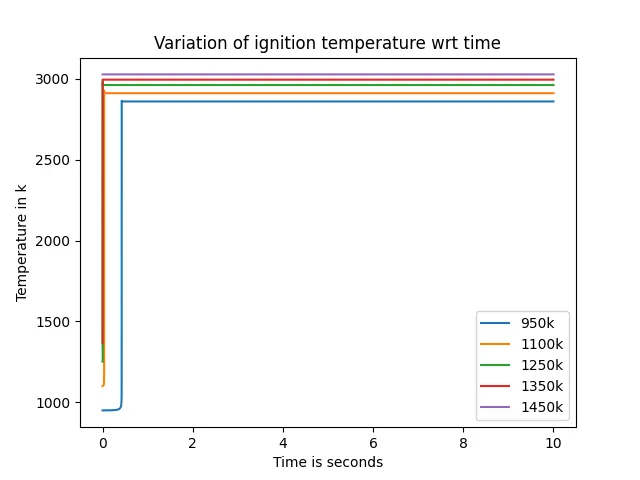
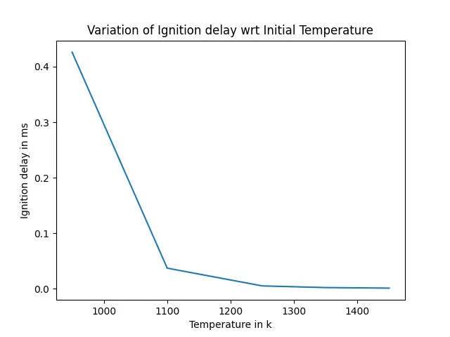
- It can be observed in the first image that the ignition time decreases with increase in temperature. Higher the initial temperature, lower is the ignition time.
- On the right, the image strengthens the above sentence. Ignition delay can be observed to decrease with increase in initial temperature.
3.3 Variation of Auto Ignition time of Methane with a constant temperature of 1250K and pressure varying from 1 to 5 atm - code:
def cv_combustion(T, P, species_concentration):

	import sys
	import cantera as ct
	import numpy as py
	import matplotlib.pyplot as plt

	methane = ct.Solution('gri30.xml')

	methane.TPX = T, P, species_concentration

	reactor = ct.IdealGasReactor(methane)

	reactor_network = ct.ReactorNet([reactor])

	states = ct.SolutionArray(methane,extra=['time_in_ms','t'])
	time = 0.0

	for a in range(10000):
		time += 1e-3
		reactor_network.advance(time)
		states.append(reactor.thermo.state, time_in_ms = time*1e3, t = time)

	return states

import cantera as ct
import matplotlib.pyplot as plt

atm = ct.one_atm

ignition_delays = []
Pressures = [atm, 2*atm, 3*atm, 4*atm, 5*atm]

#For different temperatures
states1 = cv_combustion(1250, 101325, {'CH4':1, 'O2':2, 'N2':7.52})
tmax1 = states1.T.argmax()
delay_time1 = states1.t[tmax1]
ignition_delays.append(delay_time1)

states2 = cv_combustion(1250, 2*101325, {'CH4':1, 'O2':2, 'N2':7.52})
tmax2 = states2.T.argmax()
delay_time2 = states2.t[tmax2]
ignition_delays.append(delay_time2)

states3 = cv_combustion(1250, 3*101325, {'CH4':1, 'O2':2, 'N2':7.52})
tmax3 = states3.T.argmax()
delay_time3 = states3.t[tmax3]
ignition_delays.append(delay_time3)

states4 = cv_combustion(1250, 4*101325, {'CH4':1, 'O2':2, 'N2':7.52})
tmax4 = states4.T.argmax()
delay_time4 = states4.t[tmax4]
ignition_delays.append(delay_time4)

states5 = cv_combustion(1250, 5*101325, {'CH4':1, 'O2':2, 'N2':7.52})
tmax5 = states5.T.argmax()
delay_time5 = states5.t[tmax5]
ignition_delays.append(delay_time5)

plt.figure()
plt.plot(states1.t, states1.T)
plt.plot(states2.t, states2.T)
plt.plot(states3.t, states3.T)
plt.plot(states4.t, states4.T)
plt.plot(states5.t, states5.T)
plt.xlabel('Time is seconds')
plt.ylabel('Temperature in k')
plt.title('Variation of ignition temperature wrt time')
plt.legend(['1atm','2atm','3atm','4atm','5atm'])
plt.show()

plt.figure()
plt.plot(Pressures, ignition_delays)
plt.xlabel('Pressure in pa')
plt.ylabel('Ignition delay in ms')
plt.title('Variation of Ignition delay wrt Reactor Pressure')
plt.show()
3.31 Results
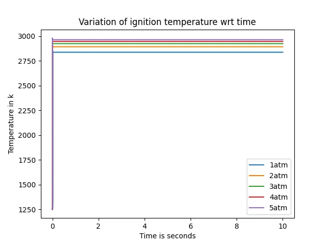
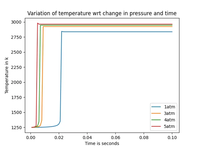
- The top left image in this section is for simulation time of 10 seconds and top right image is for simulation time of 0.1 seconds. Both the images are presentd to observe the trend more carefully.
- Similar to temperature, increase in pressure causes increase in rate of reaction. So, reduction in ignition time. This is indicated in both the images.
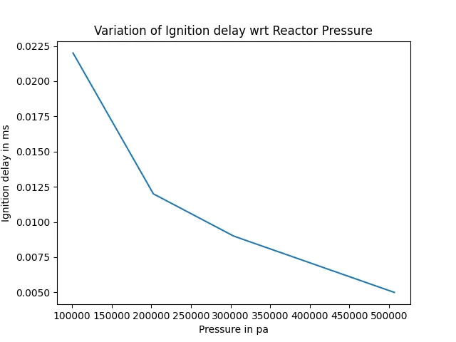
- In the last image, ignition delay can be seen decreasing with increase in pressure due to increased rate of reaction.
4. Resources: