CHT Analysis on a Graphics card

Aim: To simulate conjugate heat transfer(CHT) on the model of a graphics card and hence to:

1. Determine the maximum temperature and heat transfer co-efficient attained by the processor for the assumed value of thermal design power(TDP).
2. Perform 3 different simulations by varying velocities and mesh size.
3. Indicate the hotspots on the model due to heat dissipation.

1. Introduction:

1.1 Graphics card:

Graphics card is a part of computer hardware which makes the computer powerful by giving it the capacity to do high level works. Basically graphics card is responsible for the image that appears on monitor. Smoother and highly detailed images can be produced with a powerful graphics card.

To do such high intensity work, it needs some amount of power. While utilizing this power, the components release heat due to various reasons like power losses, due to material properties, etc. Heat can be reduced through fans, but high quantity of heat results in decreased performance. Hence, it necessary to understand where and what magnitude of heat gets released, if better performance is expected.

In this study, certain parameters are assumed, like the power consumption and materials for different components in a graphics card. Though this provides a basic understanding, similar results can be expected from a detailed analysis.

1.2 Conjugate heat transfer(CHT):

CHT is a process where heat transfer occurs majorly through both conduction and convection. For eg, in this study the heat transfer from processor to fins and to the base takes place due to conduction whereas the heat transfer from fins to the surrounding fluid takes place due to convection. Maximum dissipation can be attained only if, heat release from conduction process and convection process are maximum.

If a system only involves conduction, then the boundary condition will be the value of temperature or heat transfer co-efficient obtained by assuming constant convective heat transfer at the boundary. Similarly, in case of convection problems the boundary condition is obtained by assuming constant conduction heat transfer. But in case of conjugate heat transfer, conduction is a function of convection, which means that heat transfer near the interface is completely dependent on the convective heat transfer of the fluid.

In such cases, the boundary conditions cannot be assumed. To get accurate results, it is necessary to solve both conduction and convection simultaneously. This is where the method of conjugate heat transfer is helpful.

There are various applications which utilize the concept of conjugate process such as, energy exchange between the atmosphere and the ocean, drying of a brick or a wooden board, simple conduction between two different solids, etc. Applications of conjugate process ranges from aerospace to food processing.

1.2.1 Heat transfer processes involved:

Conduction – This is a process where heat transfer takes place due to the molecular collisions and interactions. This is governed by Fourier’s law of conduction, which states that the heat flux is proportional to temperature gradient.

`q = -k*nablaT`, where q is the heat flux in W/`m^2`, k is thermal conductivity in `W/(mk)` and `nablaT`is temperature gradient.

Convection – This is a process where heat transfer takes place due to the movement of fluid and it is governed by Newton’s law of cooling, which states that heat flux is proportional to the temperature difference between the hot and cold body.

`q = h(T_(wall) - T_(ref))`, where q is the heat flux in W/`m^2`, `T_(wall) and T_(ref)`are wall and fluid temperatures in k respectively and h is the heat transfer co-efficient in W/`m^2k`.

2. Solution approach:

To arrive at the required solution, various actions are taken and they are discussed in this section.

• Theoritical calculation is completed by assuming necessary parameters - Pwer consumption - 10watts. Thermal desing power(TDP) - 0.15625e9 `w/m^3`.
• The geometry is imported to spaceclaim and share topology is used to share all the edges, surfaces and points - This helps in conformal meshing.
• For the first case, default mesh size is used and for the next 2 case mesh size is refined by introducing method and body sizing.
• Inlet, outlet, fluid enclosure and all the different components are named.
• In fluent set-up, K-omega model is used.
• New materials from fluent database - gold and copper are defined.
• For processor - gold, base - copper, fins - aluminium, materials are selected, with a source term for processor. The calculated value of TDP is entered as the souce term value.
• Velocity is varied for all the 3 cases at inlet.
• Area-weighted average of temperature plot is defined.
• Hybrid initialization is done.
• Contours of temperature and HTC are defined.
• Solved for 150 iterations (except last case - 200 iterations).
• Results are post processed by CFD-post.

2.1 Pre-processing:

2.1.1 Geometry

The geometry is imported to spaceclaim and share topology is used to get conformal mesh. The main focus in this study is the processor and hence its physical aspects are important such as the volume - 64`(mm)^3`. Other dimensions are not very important for this analysis.

To calculate heat released, this value of volume is necessary. Heat release can be calculated through the formula for Thermal Design Power(TDP) - (Power consumption/volume).

Here power consumption is assumed to be 10watts. Therefore TDP = `(10/64) = 0.15625e9 w/m^3`.

In the below left image, the top portion represents fins which is assumed to be made of aluminium and in the right image, the top green component - processor is assumed to be made of gold and the bottom component - base is assumed to be made of copper.

The last image in this section (fig - 2.3) represents the enclosure used for the analysis.

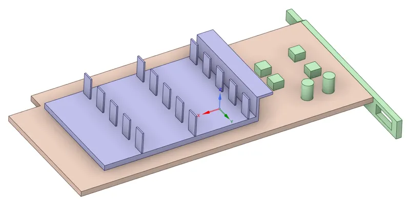
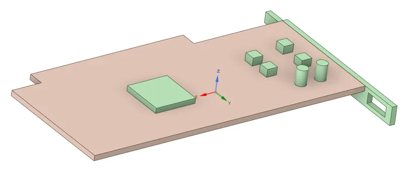
Fig - 2.1 Fig - 2.2

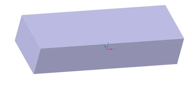
Fig - 2.3

2.1.2 Mesh

Default case - This is considered for case - 1 analysis.

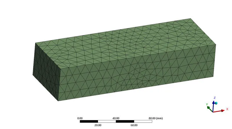
Fig - 2.4

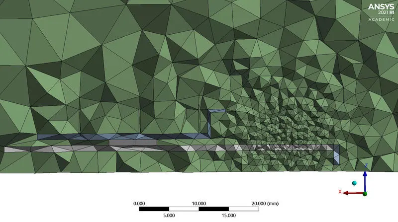
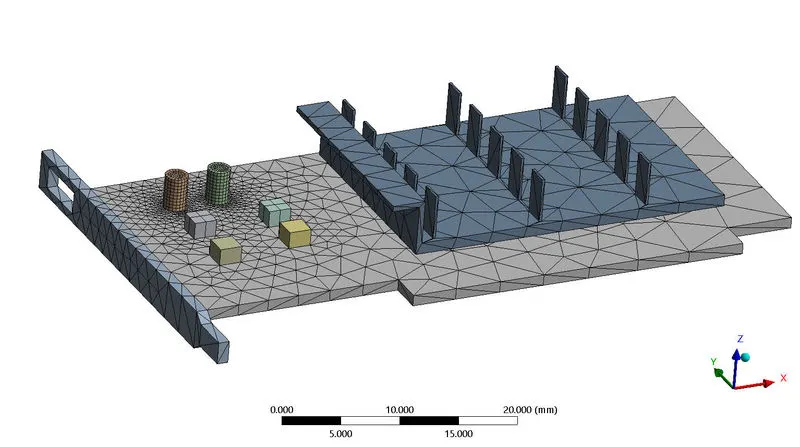
Fig - 2.5 Fig - 2.6

Refined mesh - This is considered for cases 2 and 3.

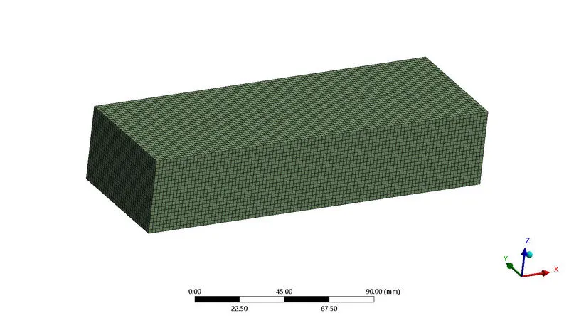
Fig - 2.7

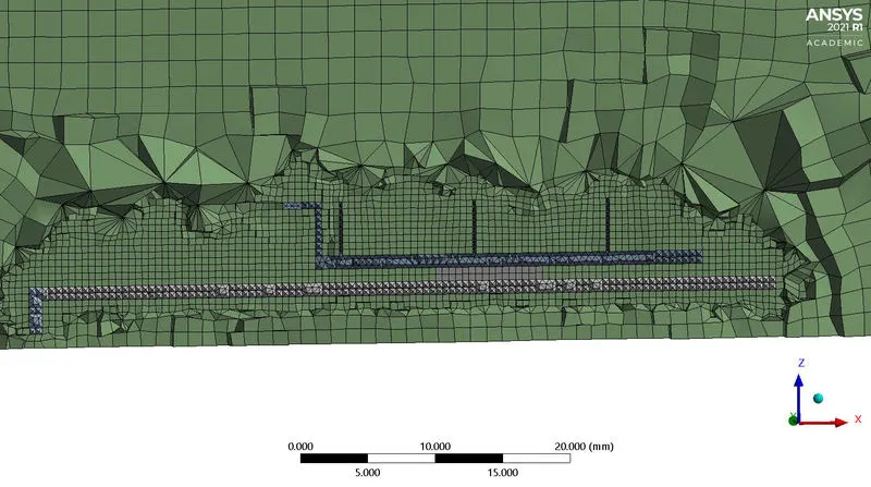
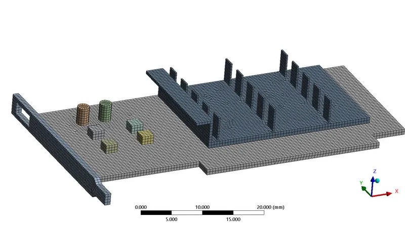
Fig - 2.8 Fig - 2.9

Mesh Details: Table - 1

Sl.No	Parameters		Details
1.	Default mesh	Number of elements	84,643
		Number of nodes	15,877
		Element size	10mm
2.	Refined mesh	Number of elements	3,89,401
		Number of nodes	2,04,635
		Method	Hex-dominated – element size – 2mm
		Body sizing	0.5 mm

• For the refined case, hex-dominant mesh is selected because hex-dominant meshes work better for wall bounded flows. In study near wall treatment is important for both temperature and HTC distributions.
• Also structured mesh executes a bit faster compared to unstructured mesh.
• And decreasing the element size increases accuracy (not much in this study).

2.2 Solver:

For this study, K-omega turbulence model is selected. Compared to k-epsilon model, k-omega model has improved accuracy and since this is a conjugate heat transfer problem, near-wall treatment becomes very important to accurately predict the temperature and heat transfer co-efficient distributions. Hence k-omega is selected.

2.2.1 Material Properties

Table - 2:

Sl. No	Material	Density (rho) – kg/m^3	Specific heat at constant pressure (Cp) – J/(kg-k)	Thermal conductivity (K) – w/(mk)
1.	Aluminium	2719	871	202.4
2.	Copper	8978	381	387.6
3.	Gold	19320	129.81	297.73

2.2.2 Boundary condition

In the BC, only the value of velocity is varied - 1m/s, 2.5m/s and 5m/s. All other parameters are kept constant.

3. Results:

3.1. Case 1: Velocity-1m/s, Mesh size - default

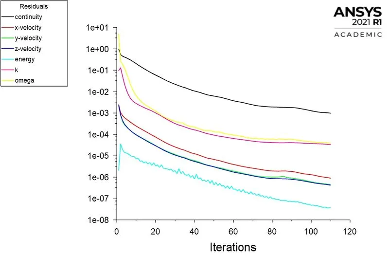
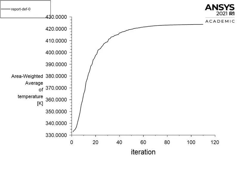
Fig - 3.1 Fig - 3.2

• For this case, the solution converged at 109 iterations. The convergence of solution can be seen in Fig - 3.2, where the temperature almost becomes a constant after around 80 iterations.
• Also the residuals have reached a very low value which can also be seen to become a constant after 80 iterations.
• The maximum temperture attained for this case is 423K.

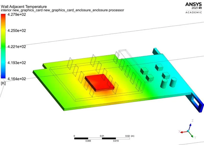
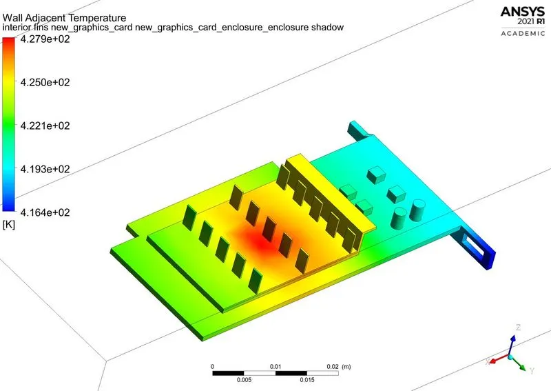
Fig - 3.3 Fig - 3.4

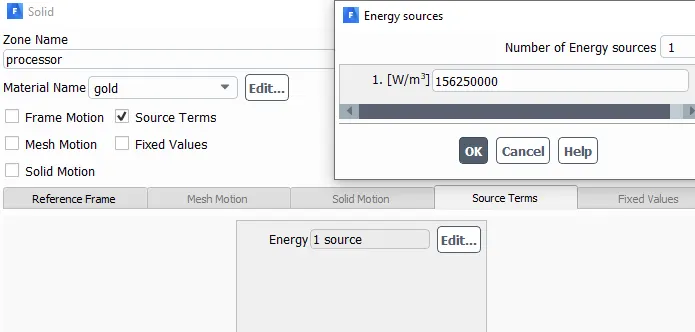
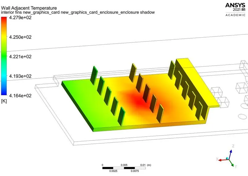
Fig - 3.5 Fig - 3.6

• In the above figures 3.3, 3.4, 3.6, the hotspots can be observed near the area around the processor. This is natural as the processor is heat source in a graphics card.
• Figure 3.5 indicates the cell zone inputs.

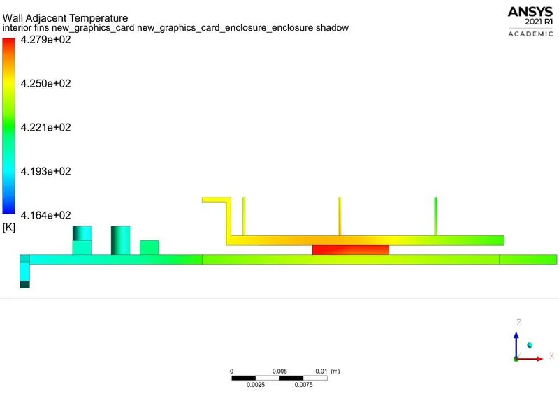
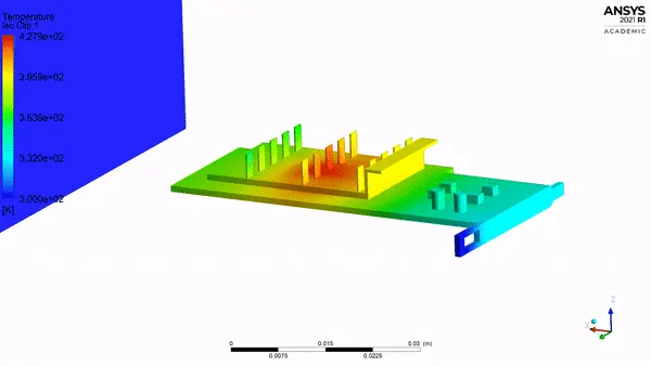
Fig - 3.7 Gif - 3.8

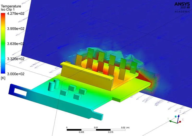
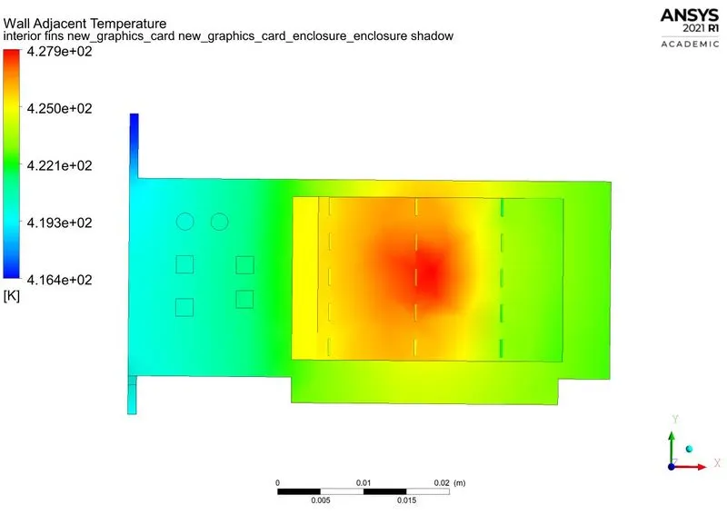
Fig - 3.9 Fig - 4

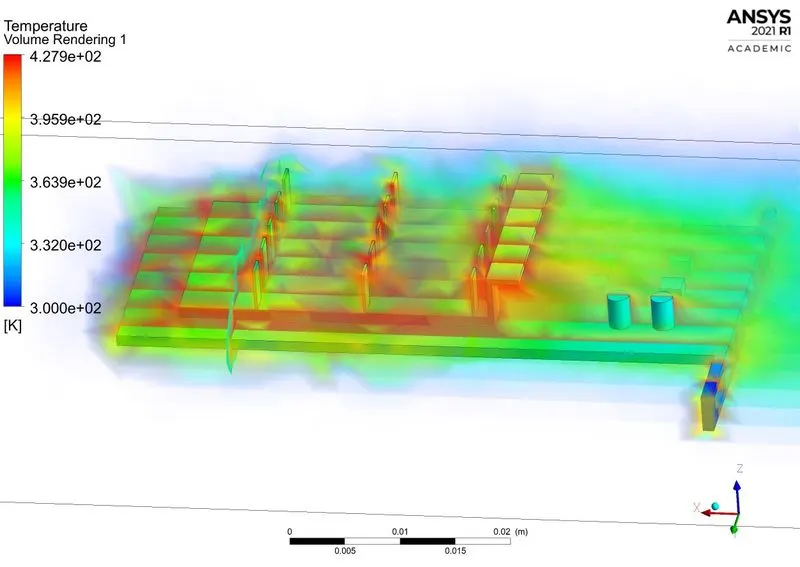
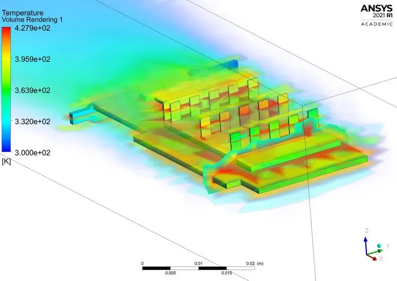
Fig - 4.1 Fig - 4.2

• Figures 4.1 and 4.2 represent volume rendering of temperature.

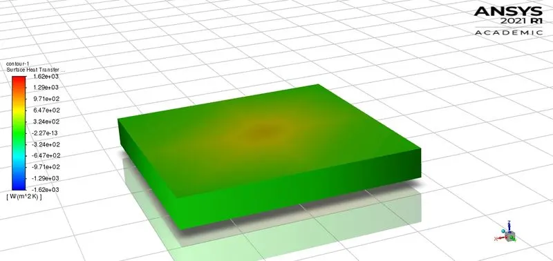
The above image indicates HTC distribution on the processor. Also the maximum value of HTC for this case is 1620W/`m^2K`.

3.2. Case 2: Velocity - 2.5m/s, Mesh - Refined:

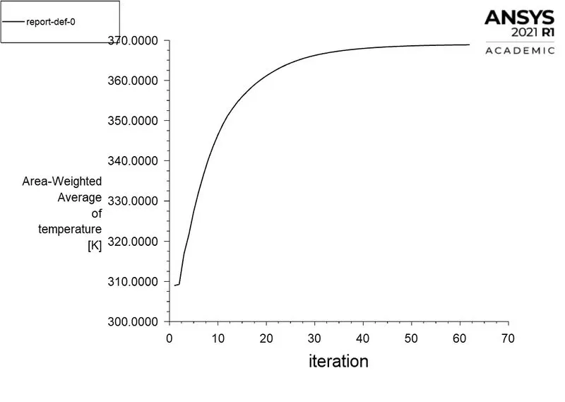
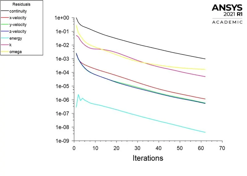
Fig - 4.3 Fig - 4.4

• In this case, convergence is achieved at 63rd iteration.
• Maximum temperature attained in this case is 373K. The reduced temperature is due to increased Reynolds number, which is due to increased velocity (2.5m/s).

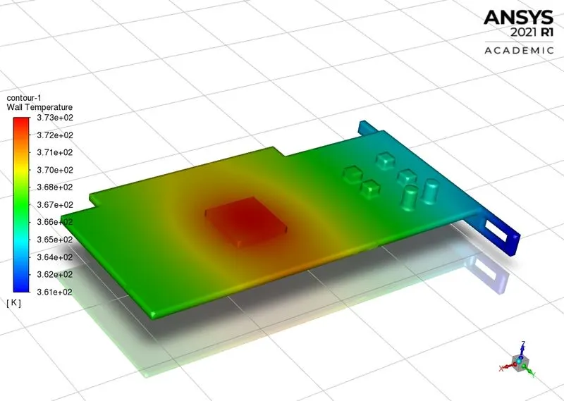
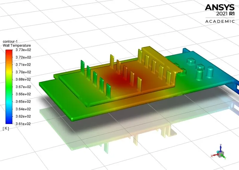
Fig - 4.5 Fig - 4.6

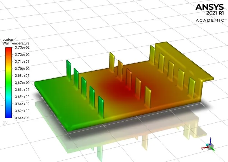
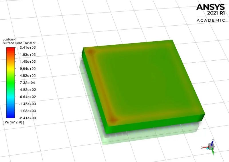
Fig - 4.7 Fig - 4.8

• Fig - 4.8 represent the surface heat transfer co-efficient distribution on the processor.
• Maximum value of HTC for this case is 2410W/`m^2K`.

3.3. Case 3: Velocity - 5m/s, Mesh - Refined

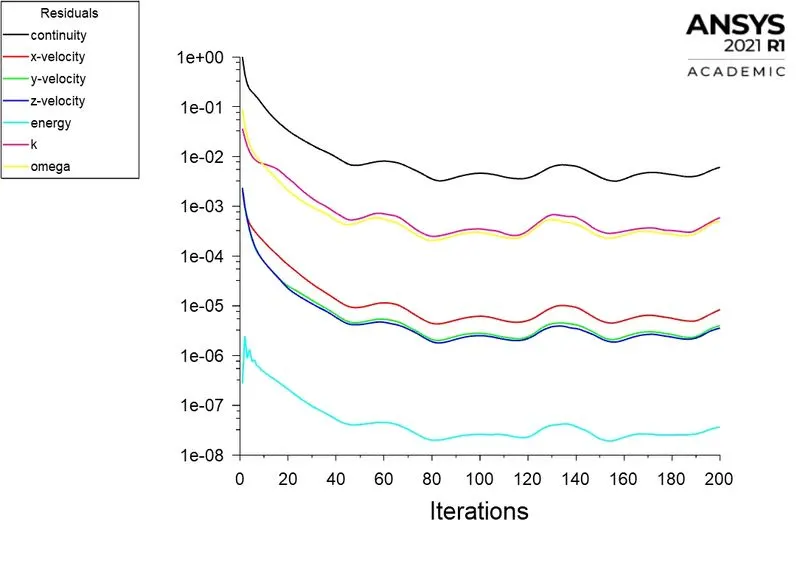
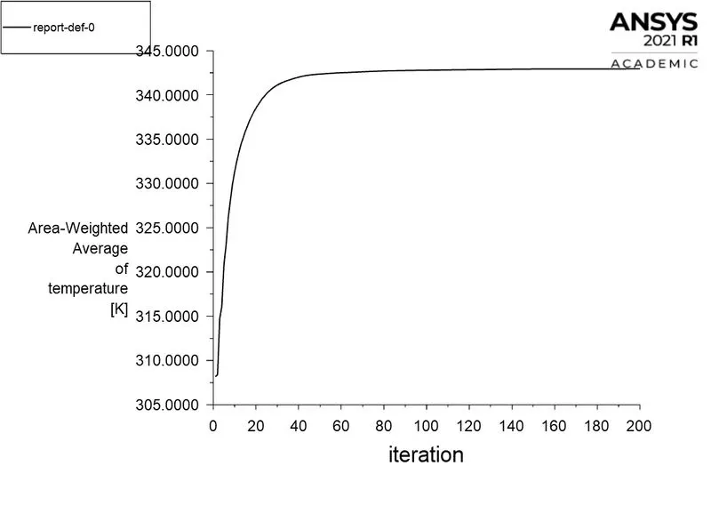
Fig - 4.9 Fig - 5

• For this case the numbers to reach convergence increased, as the residuals kept fluctuating over a number of iterations. Though there are fluctuations, in the temperature plot, temperature value becomes a constant after around 70 -80 iterations.
• Increased number of iterations in this case can be due to increased velocity. This probably induced vortex formation near the fins and hence the result.
• Maximum temperature attained in this case is 343K. This is lesser compared to the previous case as the reynolds number further increases in this case for velocity - 5m/s.

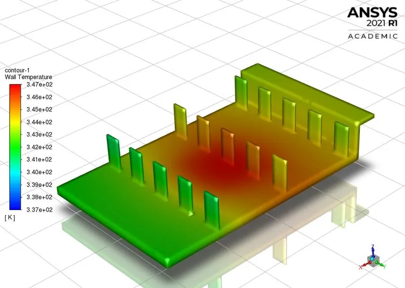
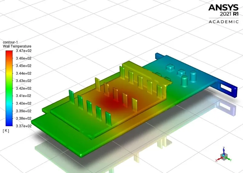
Fig - 5.1 Fig - 5.2

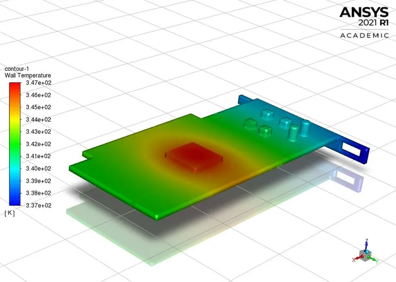
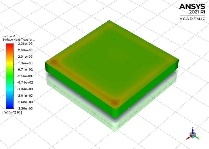
Fig - 5.3 Fig - 5.4

• Hotspots are the same as discusse earlier.
• Maximum value of HTC attained for this case is 3360W/`m^2K`.
• Increased value of HTC can be again attributed to increased velocity.

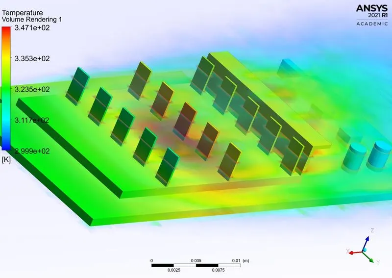
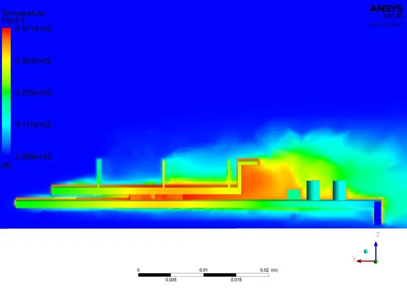
Fig - 5.4 Fig - 5.5

4. Conclusions:

• In this CHT analysis, it can be inferred from the 3 cases that increase in velocity leads reduced temperature in and around the hotspots.
• It also increases HTC,which is an attribute of forced convection.
• Number of iterations to converge decresed from case 1 to case 2 where as for case 3 it increased - probably due increase in Reynolds number.
• Changing materials for different components of the graphics card may change the values of temperature and HTC. But, the distribution remains same.