Flow simulation over MH-78 airfoil using CONVERGE CFD

Aim: To perform flow simulation over MH-78 airfoil using CONVERGE CFD for different Angle of Attacks.

1. Introduction:

Airfoils are 2D surfaces which are used to construct lift generating components such as wings, turbine blades, etc. The shape of airfoil results in lift and drag generation. It works on 3 priniciples - Bernoulli's principle, Newton's 3rd law and Coanda effect.

Bernoulli's Principle:

According this principle, increase in the kinetic energy of fluid causes decrease in the static pressure of the fluid.

`1/2*rho*v^2 + rho*g*z + P`= constant.

Newton's 3rd law:

For every action, there is an equal and opposite reaction. In aircrafts, the wings are responsible for guiding the air downwards, which makes air molecules push the wing upwards and hence generating lift.

Coanada Effect:

According to this effect, the fluid follows the curved path and remains attached to the curved path. or It is the tendency of the fluid to stay attached to the curved surface. For airfoils, this allows the flow to follow curvature of airfoils and hence the generation of lift and drag forces.

Below images represent the flow over airfoil and terminologies of airfoils.

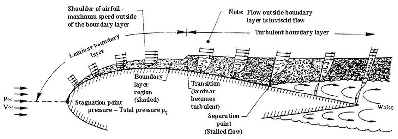
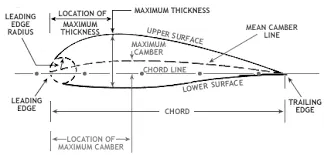
Source - Aerospace Engineering Blog

There are a few basic design definitions related to an airfoil.

• Leading edge - The front part of the airfoil.
• Trailing edge - The tail part of the airfoil.
• Chord - Length of the straight line connecting Leading edge and the trailing edge.
• Camber - The degree convexity in airfiol's cuve from leading edge to trailing edge.
• Angle of Attack - The angle between chord line of airfoil and the relative motion of fluid.

Airfoils operating in the range of 70,000 Re to 200,000 Re represent Micro-Air-Vehicle airfoils. MAVs are mentioned here because, the study is based on the Low Re reflex/thin cambered airfoil - MH-78.

To achieve optimal value of lift co-efficient and lift to drag ratio, it is important to understand the behaviour of airfoils at low Re. At low Re, the boundary layer near the leading edge is highly laminar. And hence the viscous forces dominate in this region. In this region, the flow particles have less momentum.

Due to lower momentum, these particles cannot move transversly to regions of adverse pressure gradients, which results in laminar flow separation. This forms a laminar separation bubble on the airfoil. The separation bubble length decreases with increase in Re. This separated bubble in turn forms free shear flows which causes the flow to become turbulent. The transition to turbulence is due to amplification of invisicd instabilities.

The performance of reflex airfoils at low Re is better due to the formation of short laminar separation bubble. After the separation bubble is formed, if Angle of Attack (AOA) is increased, the bubble reaches the leading edge. At a particular AOA, the bubble at the leading edge bursts and this results in stall, where lift is lost. Due to the shape of reflex airfoils, the movement of this laminar separation bubble towards leading edge is slow.

And since the operating Re is low, length of separation bubble is also less. Studies on airfoils have indicated that airfoils with shorter separation bubbles provide more lift.

Airfoils such as MH-78 or low cambered airfoils are observed to have increased lift co-efficient compared to other airfoils.

1.1 Governing equations

The flow is considered to be 2D, Compressible and the equation form is in Conservation form. Becuase the the geometry or control volume is fixed in space with fluid moving through it (control volume here is a virtual wind tunnel). Suitable boundary conditions are defined to solve the below governing equations.

The equations are given by:

• Continuity - `(delrho)/(delt) +nabla.(rhov) = 0`
• Momentum -
  • X - component - `(del(rhou))/(delt) + nabla.(rhouV) = -(delP)/(delx) + (del tau_(x.x))/(delx) + (del tau_(y.x))/(dely) + (del tau_(z.x))/(delz)`
  • Y - component - `(del(rhov))/(delt) + nabla.(rhovV) = -(delP)/(dely) + (del tau_(y.y))/(dely) + (del tau_(x.y))/(delx) + (del tau_(z.y))/(delz)`
• Energy - `del/(delt).[rho (e + v^2/2)] + nabla. [rho (e + v^2/2)*V] = rho.q + del/(delx) (K . (delT)/(delx)) + del/(dely) (K . (delT)/(dely)) - (del(uP))/(delx) - (del(vP))/(dely) + (del(vtau_(xy)))/(delx) + (del(utau_(yx)))/(dely) + (del(vtau_(yy)))/(dely) + (del(utau_(x.x)))/(delx)`

Where 'V' in energy equation is the velocity vector. V = ui+vj. Body forces are neglected.

Along with the above mentioned equations, 2 more equations are solved for Turbulent kinetic energy and Viscous dissipation rate.

2. Solution Approach:

• Geometry:
  • Airfoil co-ordinates are copied from MH aerotools website and vertices are created for every co-ordinate in Converge Studio.
  • These vertices are patched to form traingulated airfoil using patch option.
  • The same surface is copied and the edges are lofted to create a 3D surface(wing).
  • A virtual wind tunnel is created with dimensions - 50*chord length * 30*chord length and the wing is placed inside this wind tunnel.
  • The chord length of MH-78 airfoil considered is 0.1m and wing span is 0.2m, which is also the z-directional distance of virtual wind tunnel.
  • As this is a 2D simulation, a slice of the wind tunnel is considered for post-processing.
• Mesh:
  • Initially for 1degree Angle of Attack, the mesh size is 0.03m with fixed embedding.
  • For further AOAs, to observe detailed flow visualizations, adaptive mesh refinement using pressure is used.
• Solver:
  • A transient solver is used as the flow belongs to turbulent region.
  • Initially, to compare the effects of using different turbulence models, both K-epsilon and K-omega are used for 1 degree AOA and for remaining AOAs, K-epsilon model is used.
  • Boundary conditions are defined for 2D walls, symmetry walls and airfoil.
  • A region consisting of air with a certain velocity is created inside the wind tunnel.
  • Inlet velocity at the boundary is calculated using the Reynolds number. For this study, Re is 200,000.
• All the input files are exported to a folder for each case (each AOA).
• The simulation is run on 8 processors and results are post-processed using Paraview and Converge Studio's line plotting option.

3. Pre-processing:

3.1 Geometry

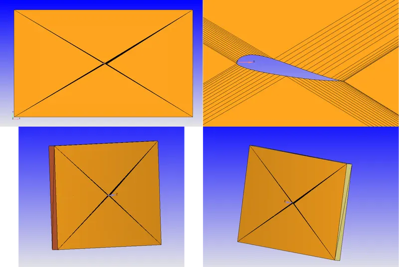
• The dimensions of the virtual wind tunnel shown above is 5m*3m*0.2m.
• The airfoil surface is created by joining all the vertices. The co-ordinates for these vertices are obtained from MH-aerotools website.
• Chord length of the airfoil is 0.1m.
• Angle of attack is changed by rotating the geometry in z-direction.

3.2 Mesh

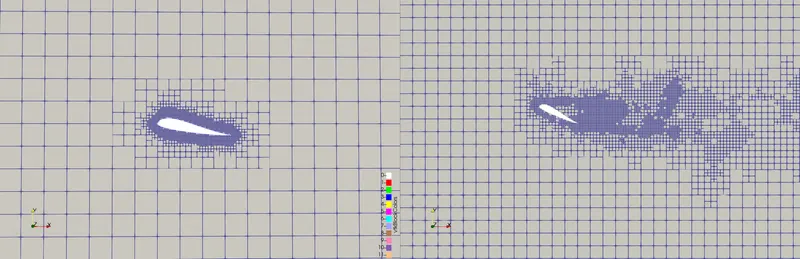
• In the above images, the left image indicates fixed embedding mesh technique and the right image indicates Adaptive Mesh Refinement.
• The base mesh size considered for all cases is 0.03m*0.03m*0.03m. But, for 1 degree AOA, fixed embedding (a method to refine areas of importance) is applied. This is done to observe the difference in visualization. Fixed embedding is suitable at lower angle of attacks where there is no flow separation.
• To simply observe the contours of flow field parameters, fixed embedding is appropriate and the details pertaining to fixed embedding is shown below.

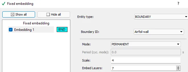
• Scale refers to the degree of refinement.
• Adaptive Mesh Refinement (AMR) is a method used to refine areas during the simulation itself. It uses the difference between curves of flow variables for refinement.
• In this study the refinement condition is set for pressure curves. The details of AMR is shown below.

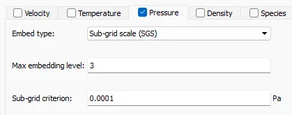
• The refinement criterion here is the difference of 0.0001 Pa in pressure curves. If the solver detects any area satisfying this criteria, it will refine the area with embedding level 3.
• AMR is very helpful to visualize areas of adverse pressure gradient. Pressure gradients exist at high AOAs and hence this method is used for all cases except 1 degree AOA.

4. Solver:

Solver set-up details
Simulation time parameters		Solver parameters		Boundary conditions
Total time in seconds	0.82	Solver scheme	PISO	Inlet	Velocity - 30.18m/s and Temperature - 300k
Min time step	1e-9s	Solver type	Density - based	Outlet	Pressure - 101325 Pa
Initial time step	1e-9s	Equation solver type	SOR	Front and back walls	2D Boundary condition
Max time step	1s	SOR relaxation	1	Top and bottom walls	Symmetry Boundary condition
Max convection CFL limit	1	Convergence tolerance	1e-5	Airoil	Wall - No slip Boundary condition

4.1 Turbulence models:

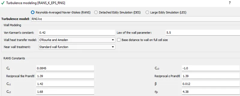
Both of the below mentioned models are of RANS type, where the flow variables are solved by using Reynolds decomposition technique. For the present study, K-epsilon model is used.

4.1.1 K-epsilon

For low Reynolds number flows, the turbulent changes near the wall are slow as the viscous forces dominate. Turbulence adjusts to these slow conditions and modelling it becomes easy. But in high Reynolds number flows, turbulent changes occur more rapidly and frequently and hence modelling this kind of behaviour is difficult.

In such cases, turbulence can be modelled by understanding the causes of turbulence from the beginning of the flow, which is the dynamics of the flow. K-epsilon model focuses on these dynamic mechanisms that alter turbulent kinetic energy.

This model solves two transport equations - one for K - turbulent kinetic energy and the other for epsilon - rate of viscous dissipation.

4.1.2 K-omega

This model also uses two transport equations to - one for K - turbulent kinetic energy and the other for omega - turbulence frequency. This model is more suited for low reynolds number applications.

5. Post-processing:

Calculations:

1. Velocity - Re considered for the study is 200,000. `Re = (rho*v*C)/mu`, where C is chord length. `v = (200,000*1.849*e-5)/(1.225*0.1) = 30.18m/s`.
2. Flow time - Length of domain = 5m and flow time = domain length/velocity = `5/30.18 = 0.16s`. The flow is made to travel 5 times and hence total flow time is 0.82 seconds.

5.1 Results for 1degree AOA

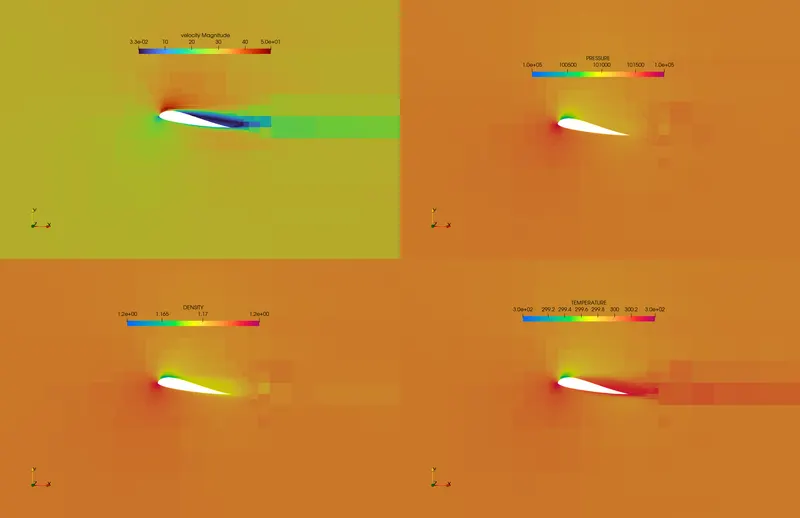
• The above image represents velocity, temperature, pressure and density distributions. In all the cases discussed below the representation remains same.
• At 1deg AOA, the laminar separation bubble can be seen near the trailing edge. At this AOA, adverse pressure gradients doesnt exist and hence the flow remains laminar and attached to the boundary layer.

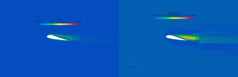
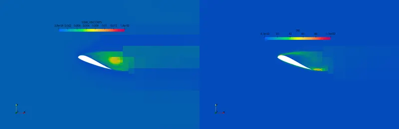
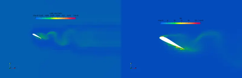
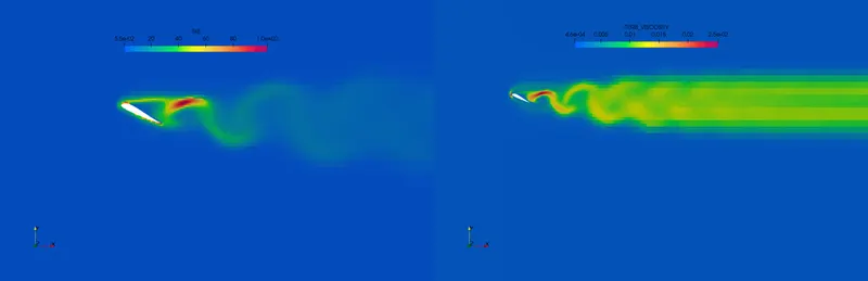
• The above results indicate that the formation of turbulent kinetic energy and dissipation of eddy viscosity are proportional. If turbulent KE increases, then the flow becomes turbulent and if viscous dissipation increases, the flow will have negative TKE. Both are not practical for 1deg AOA.

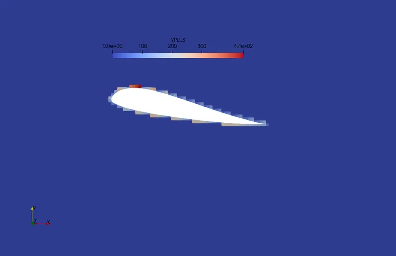
• The above image indicates the y+ contour. Y+ is non-dimensional number that represents the behaviour of flow near wall region, in this case near airfoil surface.
• The average y+ value is observed to be more than 150 and less than 250, which indicates that the flow is in turbulent log-law region.

Flow Visualization - Velocity:

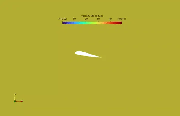
5.2 Results for 5 degree AOA

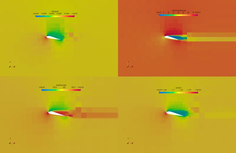
• For 5deg AOA, the length of laminar separation bubble is observed to increase. Due to this increase, small eddies form near the airfoil surface.
• The flow is mostly still attached to the surface and separation bubble moves towards to the leading edge.

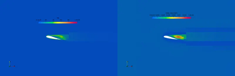
• Viscous dissipation of small eddy formed near the surface can be observed in the above image(right).

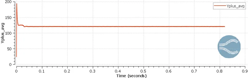
• Even for this case, y+ averages to around 120, which means the flow obeys log-law.

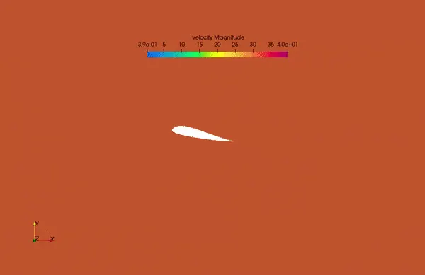
Flow Visualization - Velocity:

5.3 Results for 10 degree AOA

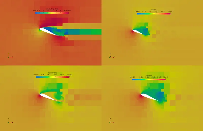
• For this AOA, the flow can be observed to be separting fully from the main flow to form strong local eddies. Even at this angle, the separation bubble is nearing the leading edge.

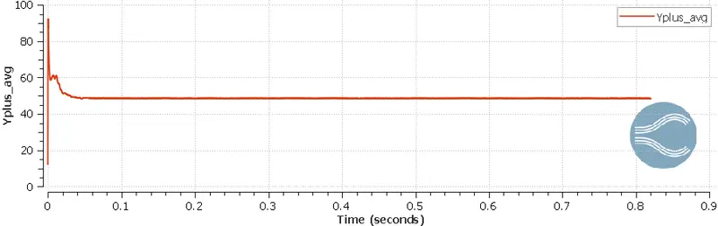
• Average y+ value for this case is around 50. This indicates that the flow is transitioning to fully turbulent flow.
• This also means that the flow near wall is still laminar and hence this is the optimal AOA for flying the aircraft.

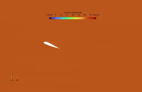
Flow Visualization - Velocity:

5.4 Results for 15 degree AOA

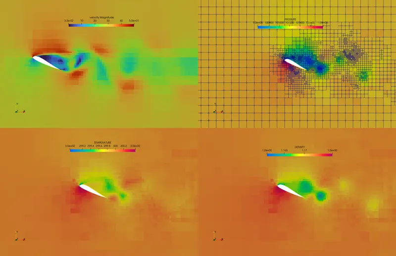
• At 15 deg AOA, the flow separation intensifies and adverse pressure gradients form outside the airfoil surface resulting in inviscid instabilities. These instabilities cause the formation of eddies.
• Initially larger eddies derive their energy from the mean flow and eventually they dissipate energy to smaller eddies and so on.
• Even at this stage, the separation bubble - in the pressure contour has not burst. So, the stall angle has not yet reached.

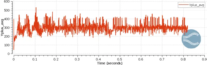
• The fluctuations in y+ values indicate that the flow is completely turbulent.

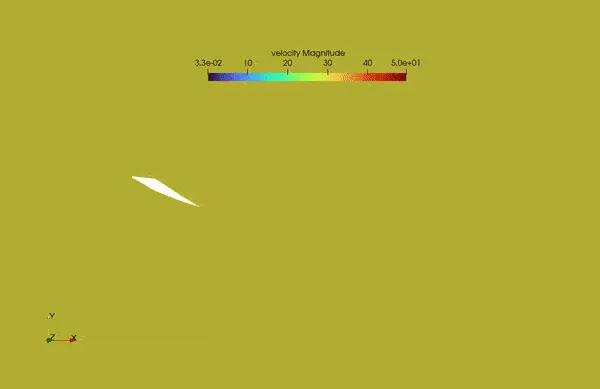
Flow Visualization - Velocity:

5.5 Results for 17 degree AOA

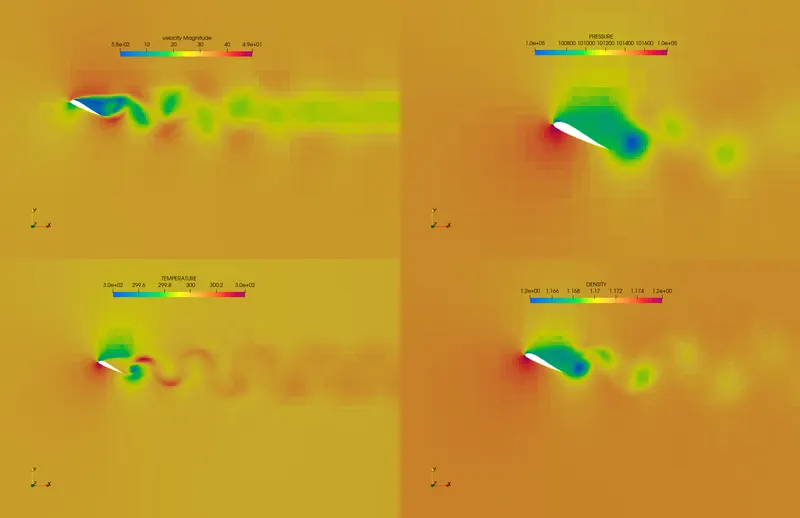
• Observe, in pressure contour above, the separation bubble has burst and transition to turbulence is compelete. Stall occurs around this AOA.
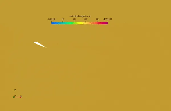
• Flow separation is intesified and clear eddies can be observed in the velocity contour.

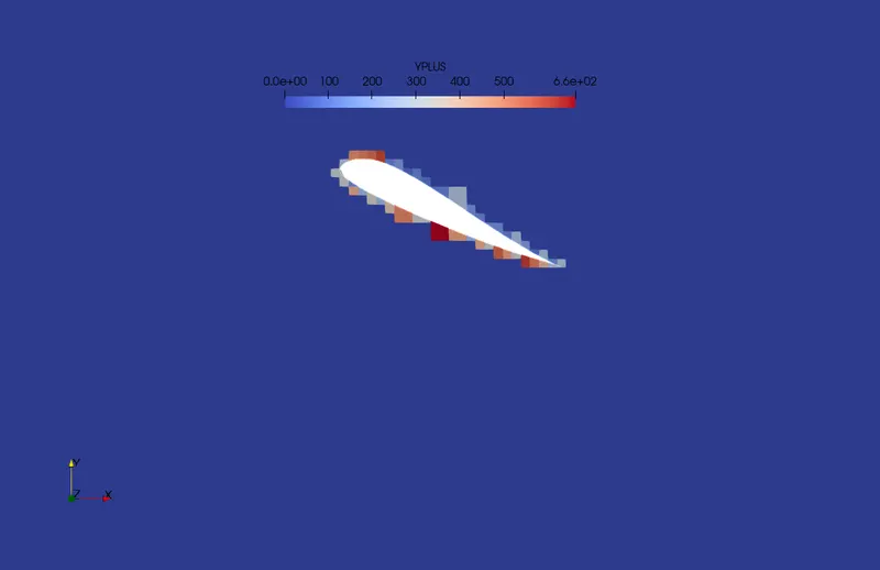
• The average value of y+ is a little more than 500, which means that the flow has reached turbulence of outer regions.

Flow Visualization - Velocity:

6. Inferences:

6.1 Lift and Drag co-efficients

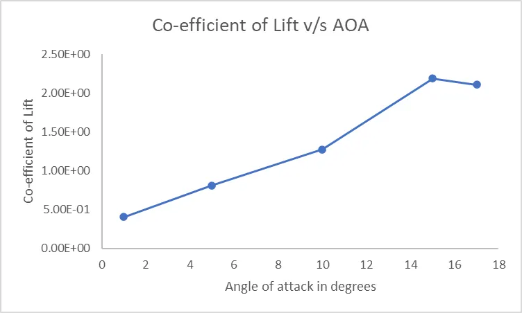
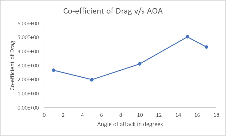
• Beyond 16deg AOA, lift falls - this condition is called stall. At this angle, the flow separates completely from the airfoil surface and results in turbulent eddies.

6.2 Variation of lift, drag, y+, TKE and viscous dissipation at all AOAs

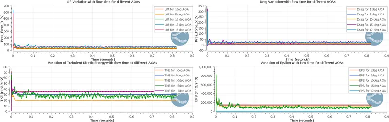
• The lift curve for 15deg AOA is on top, which means that, MH-78 at around 15deg AOA has maximum lift and after that it stalls.

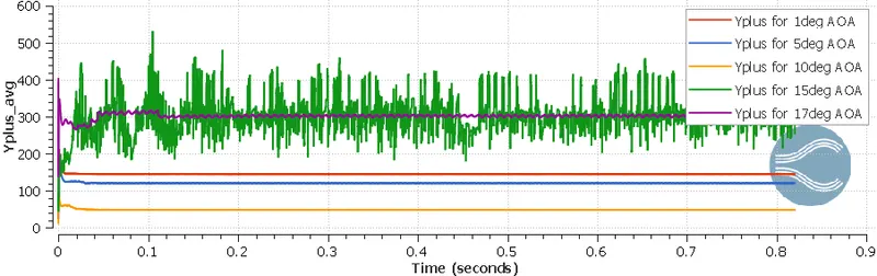
• Variation in y+ is too much for 15deg AOA, as the flow becomes completely turbulent.

6.3 Difference between use of K-epsilon and K-omega turbulence models

• Lift is slightly higher for K-epsilon and y+ values remain close for both models.
• K-epsilon is more suited for external aerodynamics applications, as it considers the mechanisms responsible for turbulence to model turbulence at high Re numbers.
• In K-omega, the turbulence modelling in high Re is based on the initial conditions. So if initial conditions are not appropriate, results will be not be realistic.

6. References:

1. https://scholarworks.rit.edu/cgi/viewcontent.cgi?article=6785&context=theses