Simulation of air flow around an Ahmed Body using CONVERGE CFD
Aim: To simulate air flow over Ahmed body using CONVERGE CFD
1. Introduction:
One of the major concerns in automobile industry is the pollution caused. This can be material wastage, emissions, etc. Collectively, all different kinds of pollutions from automobiles contribute towards global warming and many other ill effects. To counter this, it is necessary to arrive at an optimal design for the automobile. In this study car geometry has been given the focus.
Factors such drag, lift, wake, etc. are important when aerodynamic efficiency and fuel consumption are considered for any car design. Ahmed body was first proposed by Ahmed and his team in 1984. Studying this body provides us with values such as drag and lift, which can be compared with the real-world experiments and can be used to arrive at an optimal design. Although Ahmed body is a simple bluff body, it does include some features relevant to normal automobiles. For eg: the slant at the rear section of the body helps to visualize how wake varies and this can be altered by changing slant angles.
When all these factors are considered, it becomes important to study and validate the results obtained from Ahmed body.
Ahmed body is considered as a reference body to study aerodynamic parameters such as drag, lift and wake. When the resultant forces of a body are considered based on pressure, the body is termed as bluff body. For such bodies drag, lift and wake are a by product of pressure differences.
In case of Ahmed body, due to pressure difference at the front and rear section, a negative pressure is created and this increases the drag. As the body is simple in its construction and the results can be accurately matched with similar automobile bodies, this is given importance in the domain external simulation over an automobile.
1.1 Governing equations
The flow is considered to be 2D, incompressible and the equation form is in Conservation form. Becuase the the geometry or control volume is fixed in space with fluid moving through it (control volume here is a virtual wind tunnel). Suitable boundary conditions are defined to solve the below governing equations.
The equations are given by:
- Continuity - `nabla.(v) = 0`
- Momentum -
- X - component - `rho((delu)/(delt) + nabla.(uV)) = -(delP)/(delx) + (del tau_(x.x))/(delx) + (del tau_(y.x))/(dely) + (del tau_(z.x))/(delz)`
- Z - component - `rho((delw)/(delt) + nabla.(wV)) = -(delP)/(delz) + (del tau_(z.z))/(delz) + (del tau_(x.z))/(delx) + (del tau_(y.z))/(dely)`
Temperature effects are not considered and hence energy equation is neglected and Body forces are neglected.
2. Solution approach:
- Geometry
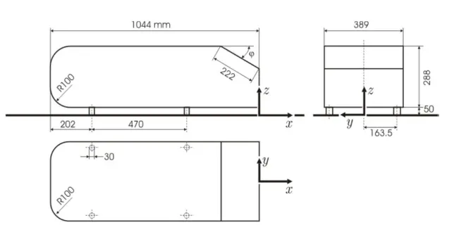
- Ahmed body is created using Solidworks for the given dimensions and saved in .stl format to import the file to Converge studio.
- A virtual wind tunnel of size 10m*3m*3m is created with the Ahmed body place at the bottom. It is placed in such a way that the boundary layer thickness is 30mm at 400mm in front of the body.
- Diagnosis is carried out to determine errors in the geometry.
- Boundaries are named for slip, no-slip, Ahmed body wall, inlet and outlet regions.
- Solver set-up
- Time based application is opted and air is defined as the pre-defined mixture.
- Transient state simulation is selected and flow is considered to be incompressible.
- Simulation time parameters are defined.
- A region with velocity 40m/s in x-direction filled with air is created.
- Boundary conditions are defined.
- K-omega turbulence model is selected.
- Grid size and fixed embedding details are defined.
- Time intervals for writing text outputs and 3D output data are defined.
- Post-processing
- Set-up files are exported to a folder. Simulation is run using 8 processors in Cygwin terminal.
- Post.h files are converted to .vtk files.
- Required results such as contours, plot over line, animations, etc are saved from paraview.
3. Pre-prcoessing:
3.1 Geometry
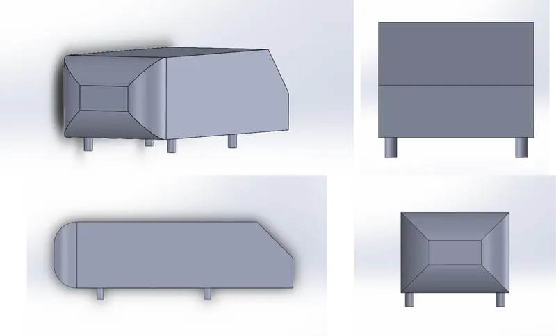
- The geometry is created using SolidWorks. The dimensions are as mentioned below.
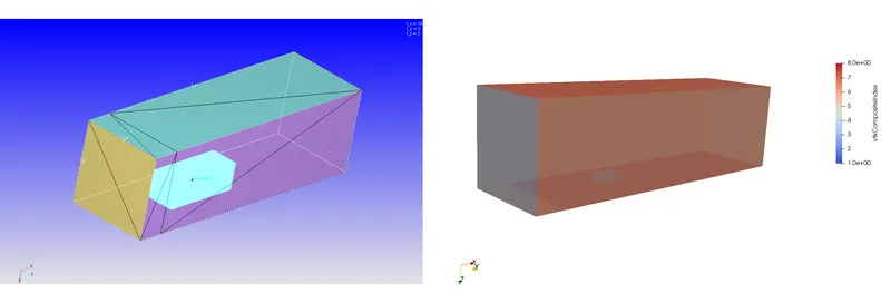
- In the above image, a small enclosure can be seen around the Ahmed body. This enclosre is created by using fixed embedding. This is to refine areas around Ahmed body to get proper visualization and accurate results.
- Also, the bottom part of the larger enclosure is divided into 2 sections. One is slip region and other is law of the wall region.
- The calculations for the distance of both regions are mentioned below.
- To match with the experimental data, the boundary layer thickness has to be 30mm at 400mm in front of the Ahmed body.
- Formula to calculate Boundary layer thickness - `del = (0.382*x)/(R_e^(1/5))`, where Re is Reynolds number.
- Velocity is considered to be 40m/s and the length term in Reynolds number is also x. So, when the above equation is solved, `x = 1.667m`
- This means that for the bottom wall to develop 30mm BLT, law of the wall BC has to enforced for 1.667m length.
- The total length in front of Ahmed body with law of the wall BC is 0.4+1.667 = 2.067m ~ 2m.
- Dimensions of the enclosure considered in x*y*z directions respectively are - 10m*3m*3m, where 1m at the beginning in x-direction has slip BC.
- For the smaller embedd box - 2.9m*1m*1m.
3.2 Mesh
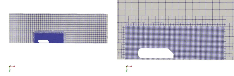
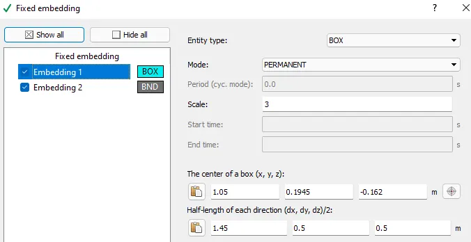
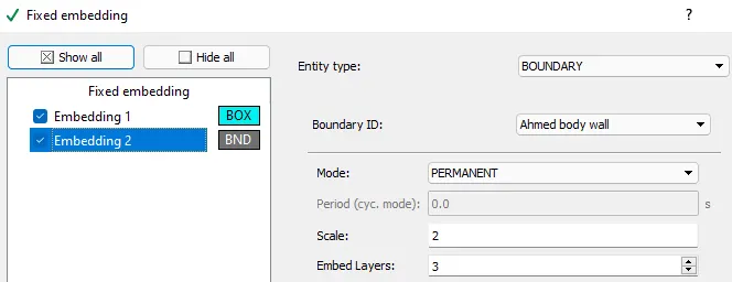
- Base mesh size considered is 0.02m and an embedding box is created around Ahmed body for accurate results. A fixed embedding is also created for Ahmed body walls. Both the embedding details are mentioned below.
4. Solver:
| Solver set-up details | |||||
| Simulation time parameters | Solver parameters | Boundary conditions | |||
| Total time in seconds | 1 | Solver scheme | PISO | Inlet | Velocity - 40m/s and Temperature - 300k |
| Min time step | 1e-9s | Solver type | Density - based | Outlet | Pressure - 101325 Pa |
| Initial time step | 1e-9s | Equation solver type | SOR | Side and Top walls | Symmetry Boundary condition |
| Max time step | 1s | SOR relaxation | 1 | Bottom No-slip wall | Law of the wall Boundary condition |
| Max convection CFL limit | 1 | Convergence tolerance | 1.00E-05 | Ahmed body | Law of the wall Boundary condition |
- Reynolds number for the flow - `R_e = (rho*v*l)/(mu) = (1.225*40*1.044)/(1.849*10^-5) = 27,66,684.69`.
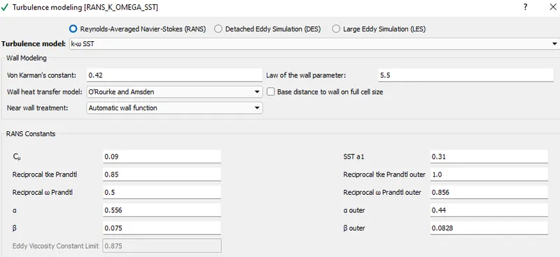
- As the flow is turbulent, a SST K-omega model is selected. This model solves two transport equations - one for turbulent kinetic energy and turbulence frequency. Turbulence frequency is used to measure the turbulene length scale.
- This model depends on the free stream conditions and since the experimental data indicate the free stream data is realistic, this model is selected.
- SST K-omega is suggested to be used for external aerodynamics applications from different experiments of performance assessments.
- The details of the model used are mentioned below.
- The flow time is calculated to be 0.25second. Fluid is made to flow 4 times through the enclosure and hence the total flow time is 1second.
4.1 Y+
- Y+ is a no-dimensional number that indicates the behaviour of the first mesh cell. Here for law of the wall BC is applied for walls, where Boundary layer develops.
- Law of the wall BC indicates the flow is turbulent near the walls and it is realistic as the Reynolds number for this study is very high.
- If no-slip BC is applied for the walls, the mesh needs to be very refined to observe the boundary layer. This increases computational requirements and hence this is also a reason for using law of the wall BC.
5. Post-processing:
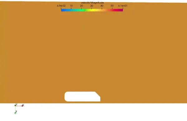
5.1 Velocity
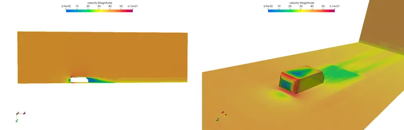
- Fluid velocity is initially high and as the fluid reaches law of the wall zones, velocity drops as the turbulent eddies derive energy from the main flow.
- The lowest of velocities is in the turbulent wake region behind Ahmed body. Here the large eddies are drawing energy from the main flow and smaller eddies are drawing energy from the larger eddies. This results in constant energy dissipation, which decreases the kinetic energy of fluid particles and hence decrease in velocity.
5.1.1 Flow visualization -Velocity:
5.2 Pressure
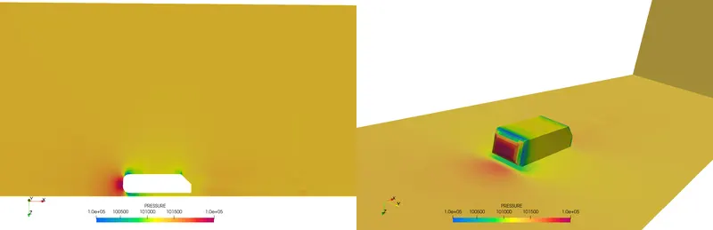
- Wake region at the rear part of Ahmed body is created due to the slant angle and adverse pressure gradient.
- Above image shows the pressure contours.
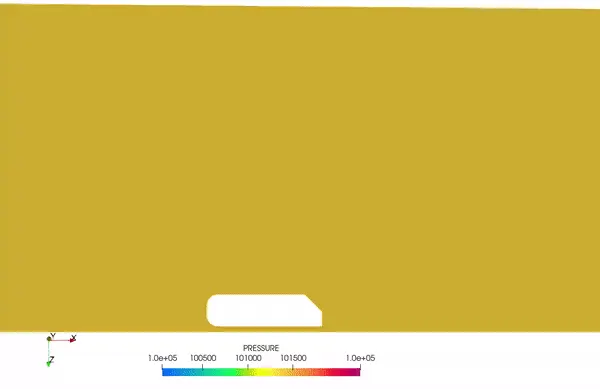
5.2.1 Flow visualization - Pressure:
5.3 Contours for Temperature, Turbulent Kinetic energy, turbulent dissipation and Y+
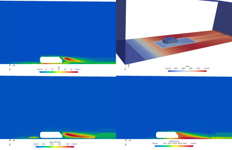
- It can be observed in the above image that TKE and turbulent disspation start instantly after slant angle and this proves the presence of negative gradient.
- Average y+ value is more than 250, which indicates that the flow is in turbulent zone.
5.5 Lift and Drag plot
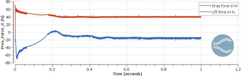
- Values of lift and drag forces after 0.5 seconds of simulation time vary constantly and hence these values are considered for calculation of co-efficient of lift and drag.
5.5 Variation of velocity at different locations around Ahmed body
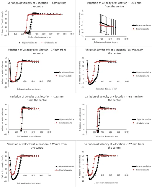
- The above image shows velocity profile for both experimental and numerical data at different x-locations.
- Small bars on black line are error bars, which are set to 5%. Some regions can have an error % of more than 5, because of the course mesh used.
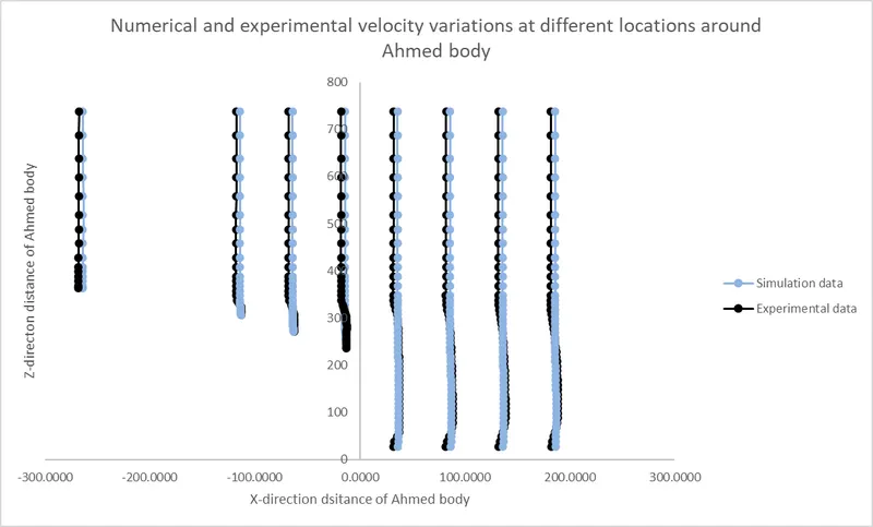
- The above image is plotted using normalized data of both experimental and numerical velocities.
- The centre of rear section of Ahmed body is considered as the origin. So there are values taken behind this origin and in front of this origin.
- Above image shows the comparison of those values.
5.6 Lift and drag calculations:
| Converge Studio calculation | Drag force in N | 39.7 |
| Co-efficient of drag | 1.19711005 | |
| Lift force in N | 15.1 | |
| Co-efficient of lift | 0.455323974 | |
| Paraview calcualtion | Drag force in N | 49.99 |
| Frontal area in m^2 | 0.03384 | |
| Co-efficient of drag | 1.507393738 |
- Drag and Lift forces are obtained by enabling wall output in Converge Studio output files section.
- Drag force from Converge studio is calculated by averaging the values for last 0.4 seconds. The frontal area of Ahmed body is determing using Paraview's extract block and extract selection options mainly.
- Once drag force and area are known - This formula is used to calcualte drag co-efficient - `C_d = (2*D)/((rho*v^2*A)`, where v is velocity in m/s, A is frontal area in m^2 and D is drag force in N.
- Similarly formula for Co-efficient of Lift - `C_l = (2*L)/(rho*v^2*A)`, where L is lift force in N.
- Drag force is calculated on Paraview using various filters such as extract block, extract surface, generate surface normals and integrate variables.
6. References: