Simulation of air flow over FSAE Car to determine the downforce and drag on all parts of the car
Aim: To simulate air flow over an FSAE car and determine the downforce and drag acting on each component for a given velocity.
1. Introduction:
The objective of this study is to understand which components contrubute towards downforce and overall drag.
When it comes to drag, there are 3 types - form drag, skin friction drag and pressure drag. Increase in drag increases the power requirements as well. Drag is primarliy caused due to the resistance offered by the surface to the moving fluid.
The car moves forward by pushing the air molecules in front of it. Air molecules resist the motion of car through them and this results in form drag. So reduced frontal area of car will have lower form drag. This is an important aspect for engine power. If form drag is lower, engine power required is also lower and the speed is higher.
Skin friction drag is what results due to the attachment of air molecules onto the surface of the car. The molecules adjacent to the surface will have zero velocity and further fluid layers will have lower velocity until the farthest layer reaches free stream velocity. This type of drag also depends on the surface roughness. All kinds of vehicles experience this drag.
The last type of drag is pressure drag. At high reynolds numbers, the flow eventually separates from the main flow due to dominating inertial forces and cause adverse pressure gradient behind the vehicle. Parts of the flow which are still laminar lack the momentum to avoid turbulence and hence these adverse pressure gradients are formed. Due to this, turbulent eddies or vortices form behind the vehicle which increases the power requirements of the vehicle.
Decreasing this eddy circulation will decrease the power requirement.
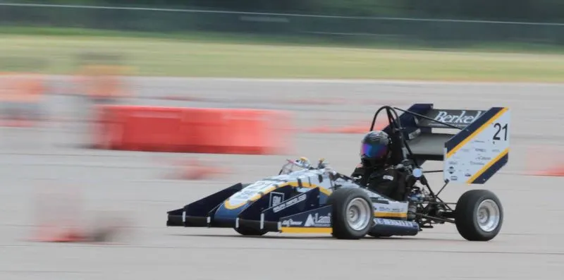
FSAE car - Source - Medium
Airfoils generate lift due to pressure difference. When airfoils are inverted they generate negative lift or downforce. This concept is used in FSAE cars to make sure tthat the entire body stays attached to the track through tires. Downforce must not be too much as it will cause difficulty in handling the vehicle. Right amount of downforce allows high cornering speeds and faster braking. It also helps in maintainin good mechanical grip between tires and the track.
1.1 Governing equations
The flow is considered to be 2D, incompressible and the equation form is in Conservation form. Becuase the the geometry or control volume is fixed in space with fluid moving through it (control volume here is a virtual wind tunnel). Suitable boundary conditions are defined to solve the below governing equations.
The equations are given by:
- Continuity - `nabla.(v) = 0`
- Momentum -
- X - component - `rho((delu)/(delt) + nabla.(uV)) = -(delP)/(delx) + (del tau_(x.x))/(delx) + (del tau_(y.x))/(dely) + (del tau_(z.x))/(delz)`
- Z - component - `rho((delw)/(delt) + nabla.(wV)) = -(delP)/(delz) + (del tau_(z.z))/(delz) + (del tau_(x.z))/(delx) + (del tau_(y.z))/(dely)`
Temperature effects and energy interactions are not considered and hence energy equation is neglected and Body forces are neglected.
2. Solution Approach:
- Geometry
- Geometry is imported to Converge studio and scaled to required dimensions.
- Geometry is checked for surface errors and errors are cleaned up.
- A virtual wind tunnel of size 35m*5m*2.5m is created around the geometry. Size of the wind tunnel is decided based on the geometry size and inlet velocity.
- All individual components such as rear wing, front suspension, body of the car, etc are named as boundaries to observe the downforce and drag.
- Turn angle -
- For case1, turn angle is 0 or the car is facing straight along x-direction.
- For case2, the average turn angle considered is `49.5^0`. The car rotates wrt z-direction.
- Mesh and Solver set-up
- Time based application is opted and air is defined as the predefined mixture.
- Initially to test and observe the physics of the problem, steady-state simulation is opted. After which, all the cases are considered to be transient.
- Simulation time parameters are defined and a region filled with air having velocity of 12.5m/s (for case1) and 20.83m/s (for case2) is created.
- Boundary conditions are defined.
- Standard K-omega turbulence is opted.
- Grid sizing, fixed embedding and grid scaling are defined.
- Time intervals for writing text outputs and 3D output data are defined.
- Post-processing
- Set-up files are exported to a folder. Simulation is run using 8 processors in Cygwin terminal.
- Post.h files are converted to .vtk files.
- Required results such as contours, mesh details, animations, etc are saved from paraview.
3. Pre-processing:
3.1 Geometry
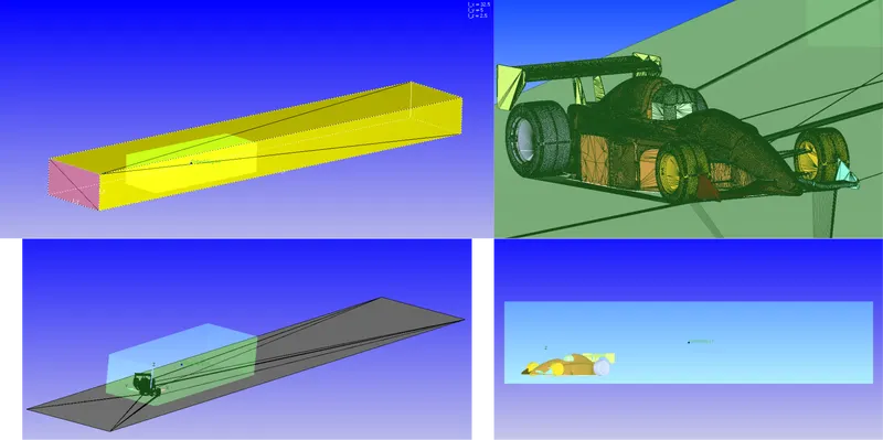
- The above images are for FSAE car with average turn angle of `49.5^0` and the light cube surrounding the car is embedding, details of which are shown in section 3.2.
- Turn angle considered is an average of -
- 70% turns at 45 degrees
- 20% turns at 80 degrees
- 10% turns at 20 degrees
- Dimensions of the car - 2.46m*1.01m*0.53m.
- The speed of the car or the average lap speed is considered to be 75kmph or 20.83m/s for case1 and 12.5m/s for case2.
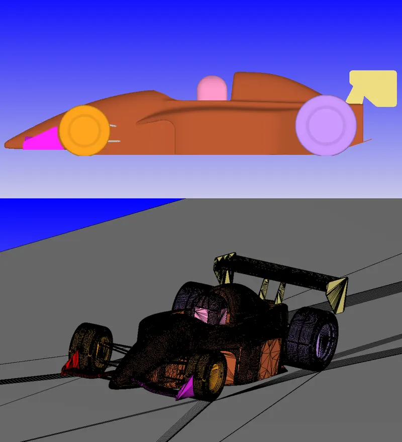
- The above images are for 0degree turn angle.
3.2 Mesh
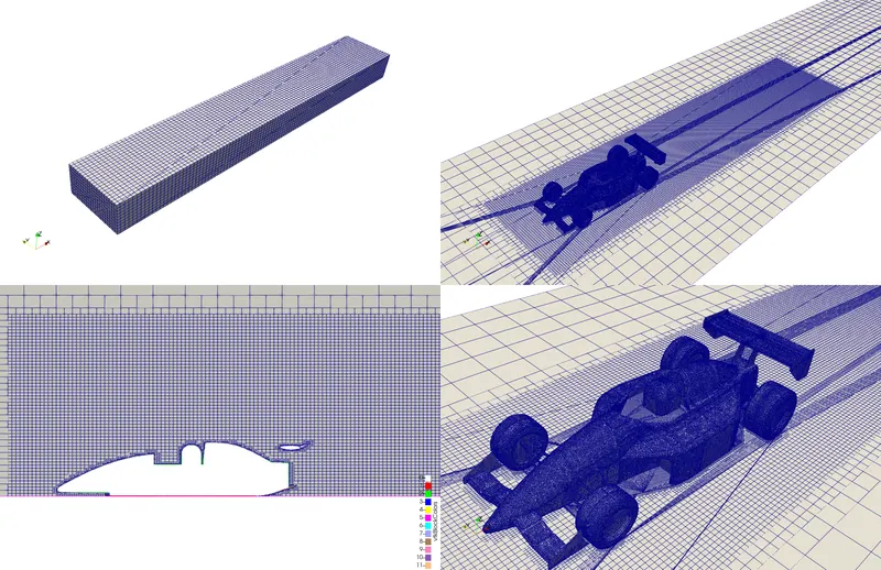
- Meshing is carried out in 3 divisions. In 1st, the virtual wind tunnel is meshed without any refinement, in 2nd the smaller enclosure around the FASE car is meshed with refinement and in 3rd the parts of FSAE car are treated as walls and refined meshing is done.
- Refinement is done to observe the wake properly.
- Y+ value of 50 is considered (Wall treatment is set to be standard). For this value of y+, first cell size is found to be 1.45mm.
- Maximum embedding scale is considered to be 5 and hence base mesh size becomes - `1.45^5 = 6.5mm`.
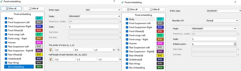
- For all parts embedding scale considered is 5 and embedd layers are 8, including for the box embedding. Fixed embedding details are shown above.
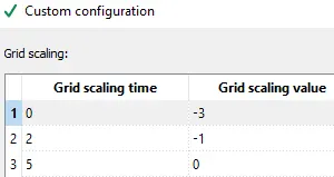
- Formula for grid scaling - `dx_(basemesh)/(2^(gridsca l e)`. Base mesh size for this study is 6.5mm and grid scaling values are shown above.
- Grid scaling is done to avoid too much load on the processors.
- For this study, for a time range of 0-2 seconds, the grid is course and from 2-5 seconds, the grid course compared to base mesh by a factor of 2 and from 5 seconds till end time, the grid is refined according to fixed embedding.
4. Solver:
| Solver set-up details | |||||
| Simulation time parameters | Solver parameters | Boundary conditions | |||
| Total time in seconds | 10 | Solver scheme | PISO | Inlet | Velocity - 20.83 m/s for case1 and 12.5 m/s for case2 |
| Min time step | 1e-7s | Solver type | Density - based | Outlet | Pressure - 101325 Pa |
| Initial time step | 1e-7s | Equation solver type | SOR | Individual components of FSAE car | Law of the wall Boundary condition |
| Max time step | 1s | SOR relaxation | 1 | Side wall of outer enclosure | Symmetry Boundary condition |
| Max convection CFL limit | 1 | Convergence tolerance | 1.00E-05 | Bottom wall of outer enlosure | Law of the wall Boundary condition |
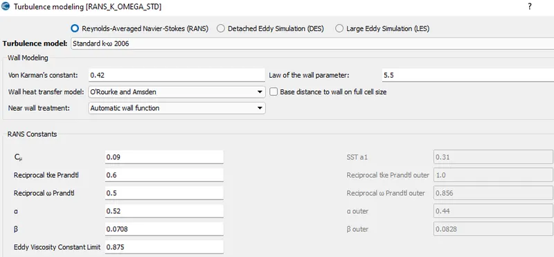
- As the flow is turbulent, Standard K-omega model is selected. This model solves two transport equations - one for turbulent kinetic energy and turbulence frequency. Turbulence frequency is used to measure the turbulene length scale.
- SST K-omega is suggested to be used for external aerodynamics applications from different experiments of performance assessments.
- Reynolds number for the flow -
- case1 - 20.83 m/s - `R_e = 3564986.86`
- case2 - 12.5 m/s - `R_e = 2139334.41`
- The flow time is calculated to be 2.52 seconds. Fluid is made to flow 4 times through the enclosure and hence the total flow time is 10 seconds.
- Details of the turbulence model is shown below
5. Post-processing:
5.1 Case1 - No turn
5.1.1 Velocity contours:
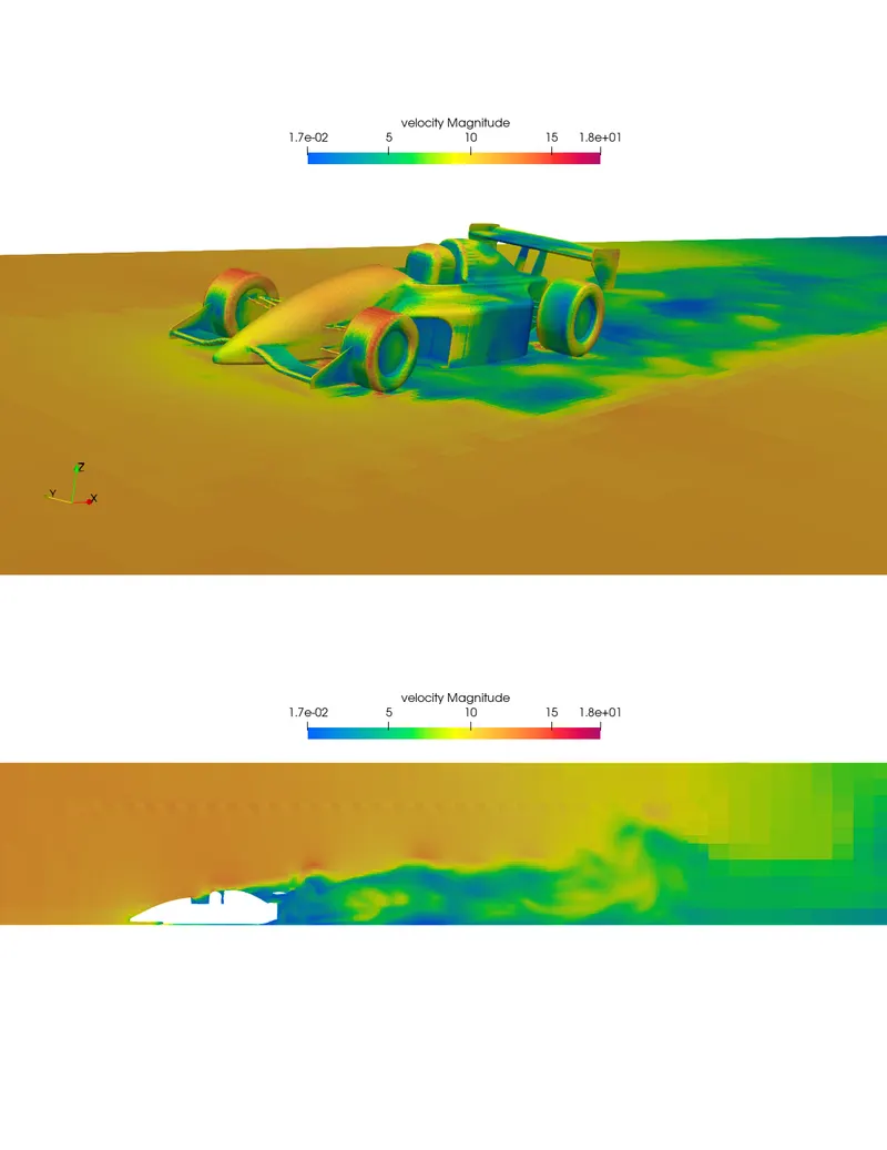
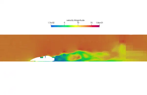
- The transition point can be observed to be just behind the helmet or human. Beyond this point, the flow separates due to adverse pressure gradient and low momentum of laminar boundary layer fluid particles.
- Behind the vehicle exists low pressure regions, where fluid velocity is higher. This results in the formation of eddies or wake region. Eddies increase the drag co-efficient and hence decrease the overall performance of the vehicle.
- Velocity distribution at different parts of the vehicle is shown in the above image.
5.1.2 Turbulent Kinetic Energy(TKE):
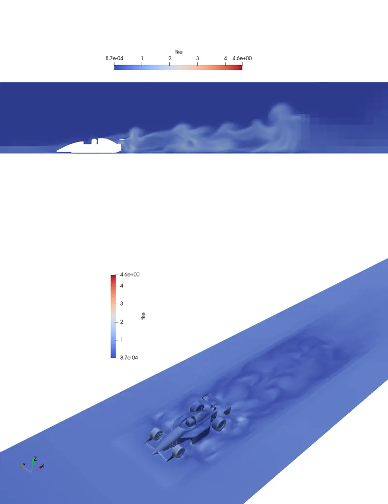
- Increase in TKE is due increase in inertial forces. This creates a low pressure high velocity region where diffusion, mixing and momentum transfer are very high among fluid particles.
- This creates a region with less drag. If this vehicle is participating in a race, then there will be other vehicles behind and a low drag region will favour other vehicles.
- TKE is calculated using turbulence models, in this case standard K-omega model.
- The contours of TKE are shown in the above images.
5.1.3 Y+ and vorticity:
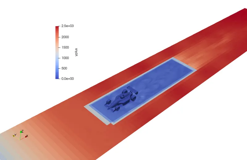
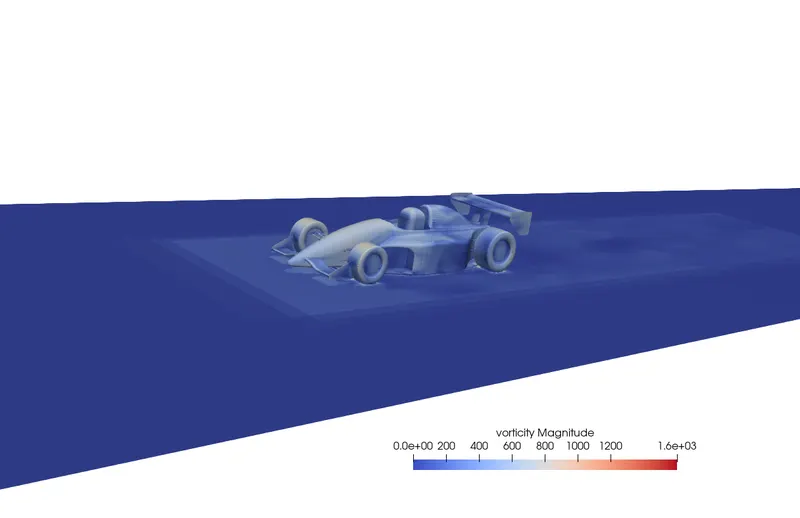
- Y+ near the wall regions is observed to be more than 200, which indicates that the flow is turbulent and resonates with law of the wall of boundary condition.
- Vorticity is the measure of local rotations of fluid particles. The contours of vorticity around FSAE car is shown above.
5.1.4 Flow visualization - Velocity:
5.1.5 Downforce
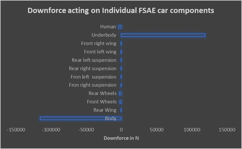
- Clearance between the underbody of the vehicle and ground in important for maintaining sufficient downforce.
- When fluid flows through constricted regions, it results in reduced static pressure and increases fluid velocity. This effect is called Venturi effect.
- Venturi effect can be seen between the underbody and ground.
- Value of downforce is positive for underbody because pressure is lower between ground and underbody. High pressure region exists above and hence the air molecules move towards the underside generating high amounts of lift. This lift presses the vehicle body against the ground, resulting in higher downforces.
- Also negative value of downforce on the body helps the vehicle maintain strong grip with the track.
- It can also be seen that other component generate compartively less downforce.
5.1.6 Drag Force
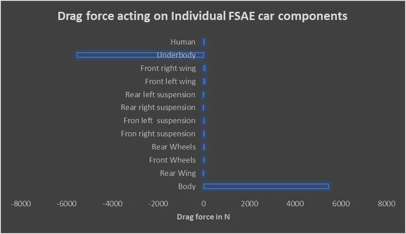
- Drag force generated by the underbody is negative because of the low pressure region between underbody and the ground.
- Due to the shape of the car body, it is generating high drag forces and this can be solved by using more optimized design.
- Other components such as front and rear wing are also generating some amount of drag and this can be solved by selecting low drag airfoils.
5.2 Downforce and drag force for a race with turns - Average turn angle - `49.5^0`
5.2.1 Downforce
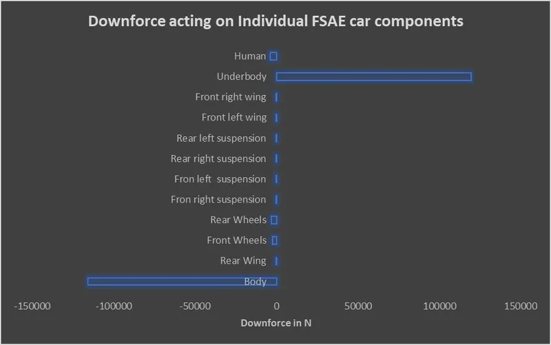
- Even for a turn angle of 49.5 degree, the downforce remains the same.
5.2.2 Drag Force
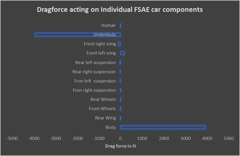
- The only change in drag force is with the front wings. Due to turn angle, front wing on the left side experiences more drag compared to right wing.
6. References: