Conjugate Heat Transfer analysis on Exhaust Port

Aims of the study:

• To simulate conjugate heat transfer (CHT) analysis on Exhaust port.
• To maintain the y+ values according to the turbulence model and justify the results.
• To calculate wall heat transfer coefficient.
• To explain the velocity and temperature contours.
• To verify the results obtained from this simulation.

1. Introduction

1.1 why and where a CHT analysis is used?

Heat transfer problems commonly involve one or two of the three heat transfer processes - conduction, convection, radiation. Problems which involve more than one mode of heat transfer are termed as Conjugate heat transfer problems.

If a system only involves conduction, then the boundary condition will be the value of temperature or heat transfer co-efficient obtained by assuming constant convective heat transfer at the boundary. Similarly, in case of convection problems the boundary condition is obtained by assuming constant conduction heat transfer. But in case of conjugate heat transfer, conduction is a function of convection, which means that heat transfer near the interface is completely dependent on the convective heat transfer of the fluid.

In such cases, the boundary conditions cannot be assumed. To get accurate results, it is necessary to solve both conduction and convection simultaneously. This is where the method of conjugate heat transfer is helpful.

There are various applications which utilize the concept of conjugate process such as, energy exchange between the atmosphere and the ocean, drying of a brick or a wooden board, simple conduction between two different solids, etc. Applications of conjugate process ranges from aerospace to food processing.

Conjugate heat transfer involves heat transfer processes where one process is dependent on the other and vice versa. Similarly in a two-system problem, if the outcome or results is dependent on both the systems, then such a problem can also be termed as conjugate.

There are also some problems which are inherently conjugate such as peristalic flow - interaction between a flexible wall of a channel and fluid inside the channel. Best example for such a case is the flow of blood inside blood vessels. By understanding such methods first hand, artificial devices such as heart lung machine can be produced. It is important to understand the process first and then practically implement it in such problems where more than kind of heat transfer is responsible for the results.

There are different methods to solve CHT problems. In this study the method of iterations is used. In this approach the first iteration provides boundary condition and based on this condition, further solution will be obtained. Convergence and accuracy depend on this boundary condition.

1.2 Types of heat transfer involved

Conduction – This is a process where heat transfer takes place due to the molecular collisions and interactions. This is governed by Fourier’s law of conduction, which states that the heat flux is proportional to temperature gradient.

`q = -k*nablaT`, where q is the heat flux in W/`m^2`, k is thermal conductivity in `W/(mk)` and `nablaT`is temperature gradient.

Convection – This is a process where heat transfer takes place due to the movement of fluid and it is governed by Newton’s law of cooling, which states that heat flux is proportional to the temperature difference between the hot and cold body.

`q = h(T_(wall) - T_(ref))`, where q is the heat flux in W/`m^2`, `T_(wall) and T_(ref)`are wall and fluid temperatures in k respectively and h is the heat transfer co-efficient in W/`m^2k`.

2. Approach:

1. Import geometry to spaceclaim and use volume extract option to create the fluid volume inside the exhaust port.
2. Share the interface using share topology option in spaceclaim to get conformal meshing.
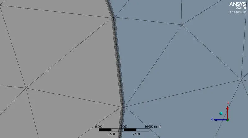
3. Mesh - initially default and for the refined version, reduce the element size and add inflation layer.
4. Create named selections - inlet, outlet and wall.
5. In fluent, select pressure based solver and steady method.
6. Select appropriate turbulence model(K-omega).
7. Define a report for surface heat transfer co-efficient(Area weighted average).
8. Initialize the flow field and create a temperature contour and solution animation.
9. Enter the number of iterations and solve.
10. Post-process the results in CFD-post and observe wall heat transfer co-efficient contour.

2.1 Pre-processing:

2.1.1 Geometry

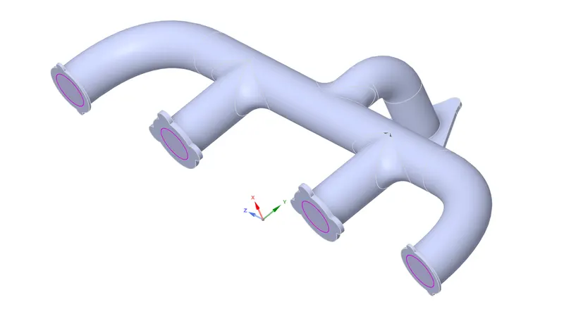
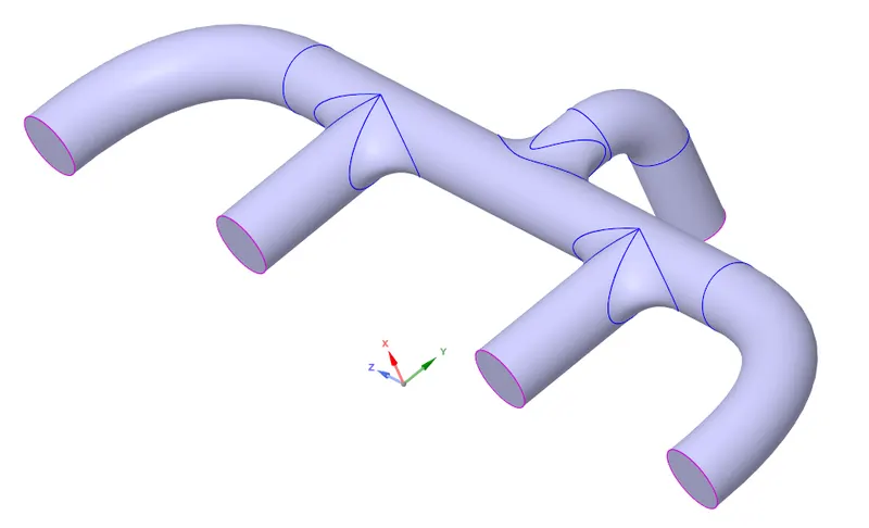
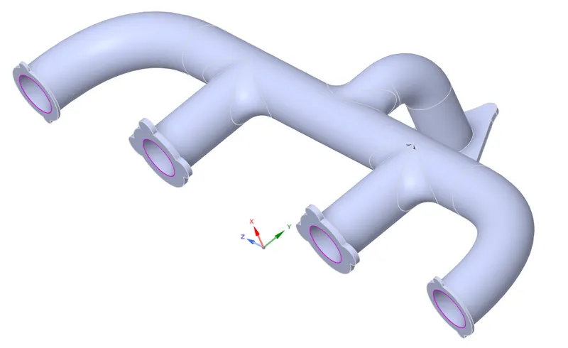
The geometry was imported to spaceclaim and using the extract volume option, the fluid volume was created. To create conformal mesh, this volume was shared with the outer layer using share topology. The outer diameter is 240mm and inner diameter is 170mm with the wall thickness 50mm.

2.1.2 Mesh

The mesh input parameters are listed in the table below.

Mesh Details
Sl. No	Mesh parameter	Input	Statistics
1.	Element size	18mm	Number of elements – 4,36,212
2.	Capture curvature min size	0.1mm	NA
3.	Inflation option	First layer thickness	NA
4.	First layer height (y)	0.0525mm	NA
5.	Maximum layers	5	NA
6.	Growth rate	1.2	NA

- Table 1

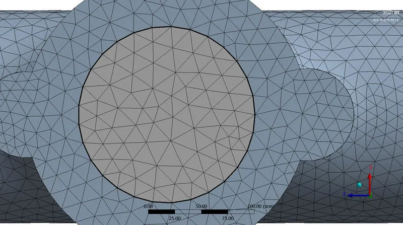
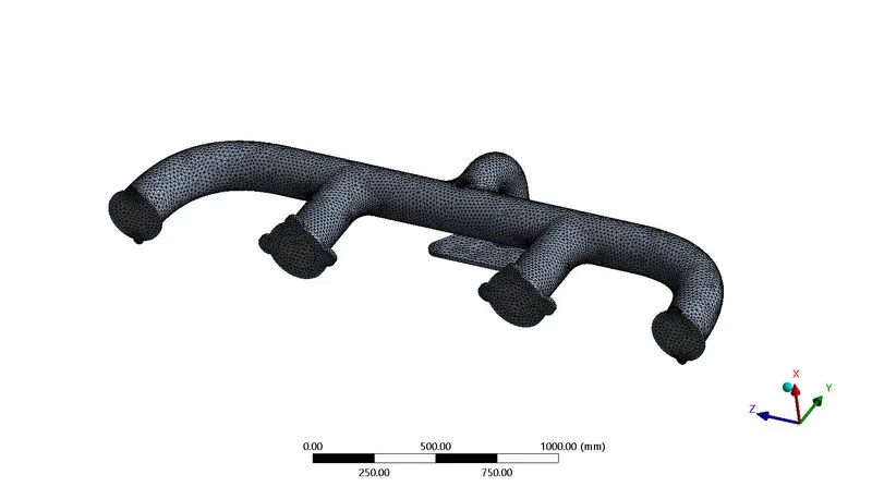- Fig 1 - Overall Mesh Representation

- Fig 2 - Inflation layer

- Fig 2.1 - Inflation layer

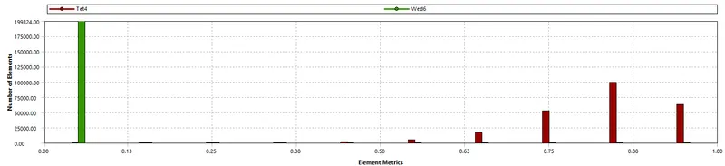- Table 2 - Element quality

2.2 Solver:

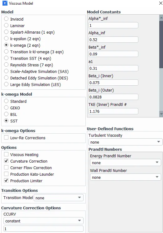
For this study, K-omega turbulence model was selected. Reynolds number for the flow was found to be 56,314, which indicates that low Reynolds number turbulence model needs to be selected. Also, internal flow and heat transfer are important parameters in this study.

Compared to k-epsilon model, k-omega model has improved accuracy for internal flows where curvature is present. Since this is a conjugate heat transfer problem, near-wall treatment becomes very important to accurately predict the temperature and heat transfer co-efficient distributions. So, the viscous sub-layer needs to be integrated with the flow and hence the mesh needs to be resolved for y+<1.

By considering all the above mentioned details, k-omega model was chosen.

2.2.1 First layer thickness calculation

Sl. No	Inputs	Values	Calculated parameters	Values
1.	Density	1.225`(kg)/(m^3)`	Reynolds number	56,314
2.	Velocity	5m/s	Skin friction co-efficient	0.0066
3.	Dynamic viscosity	1.849e-5 (at`25^0C`)	Wall shear stress	0.101N
4.	Diameter	170mm	First layer thickness	0.0525mm

- Table 2

2.2.2 Boundary conditions

Sl. No	Inlet	Outlet (outlet wall convection)
1.	Velocity – 5m/s	Thermal condition – Convection
2.	Temperature – 700k	Heat transfer co-efficient – 20w/`m^2`k

- Table 3

3. Results:

Residuals:

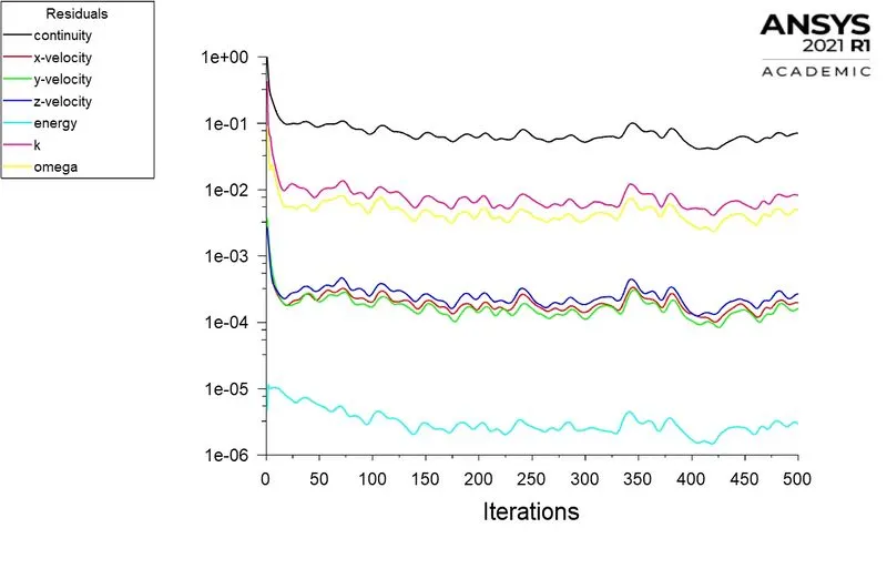- Fig 3 - Residuals

• Number of iterations - 500. Convergence achieved - at around 130 iterations.

Heat transfer co-efficient plot:

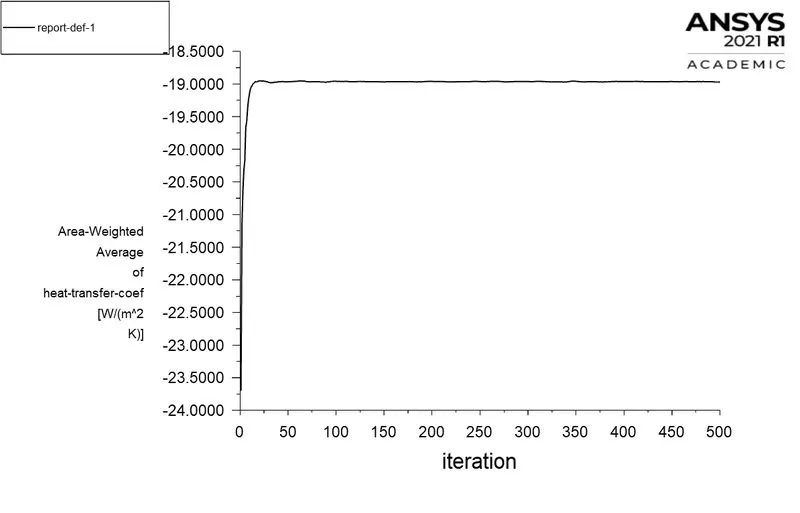- Fig 4 - HTC plot

• The above plot is for the heat transfer co-efficient on the internal solid surface of the exhaust port. The Numerical value result is 18.788 W/`m^2k`. To verify this result, below calculation is done. Near the wall, the heat will be transferred from the fluid to solid wall through forced convection and this heat transfer is important in CHT analysis.
• To analytically calcualate the HTC(Heat Transfer Co-efficient), Dittus-Boelter correlation is used. This is because of the conditions which this study satisfies.

The conditions to the correlation are - `Re >=10,000`and `0.7<=Pr<=160`. For this problem, Re is 56,314 > 10,000.

Prandtl number(Pr) is a dimensionless number which corelates the visocity of a fluid to its thermal conductivity. It can also be used to determine which among mometum diffusivity and thermal diffusivity is greater for a given fluid. It mathematical co-relation is given by:

`Pr = (C_p*mu)/k`, Where `C_p`is the specific heat of constant pressure of the fluid, `mu`is the dynamic viscosity in `pa.sec`and k is the thermal conductivity in `W/(mk)`.

Dittus-Boelter correlation is : `Nu = 0.023 * Re^(4/5) * Pr^n`, Where n is 0.4(for heating).

Calculation:

For air `C_p = 1`kj/kg, `mu = 1.872*10^-5 (kg)/(ms)` and k = `0.02588`W/mk`. After calculation, Pr = 0.72, Nu = 127.39 and h = 19.39W/`m^2k`.

So the difference between analytical and numerical values is 0.03104 and the error % is 3.1. The error is within the acceptable range and hence the numerical results indicate good accuracy of the results.

y+ distribution with respect to position of X-axis:

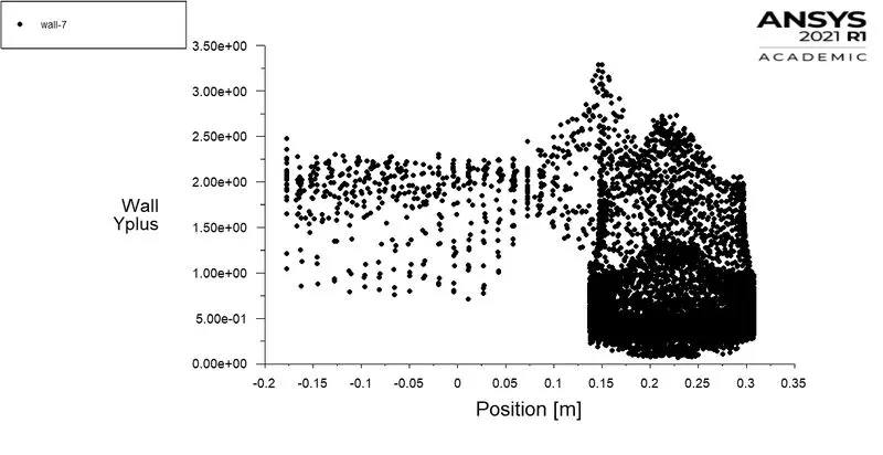- Fig 5 - y+ plot

• As mentioned in the solver section, for this problem, viscous sub-layer is important and hence y+ value has to be <5. For the model selected(k-omega), the y+ value should be <1.
• Based on this the y+ value of 1, first layer thickness was determined.
• After the convergence, above y+ plot was plotted. So, it can be observed that at any given position, y+ values do not exceed 5 and near the wall regions, y+ is fairly close to 1.
• This co-relation indicates the justification of results with the inputs.

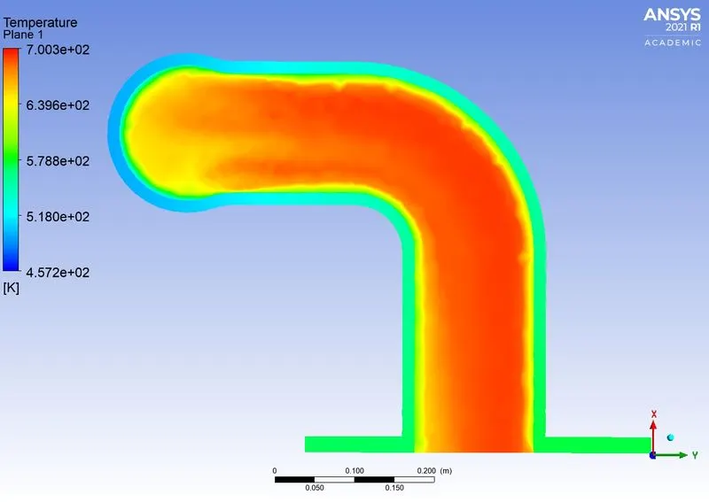
3.1 Temperature Distribution:

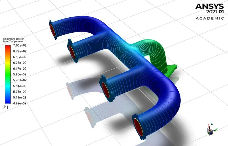- Fig 6 - Temperature contour

- Fig 6.1 - Temperature contour

3.2 Velocity Distribution:

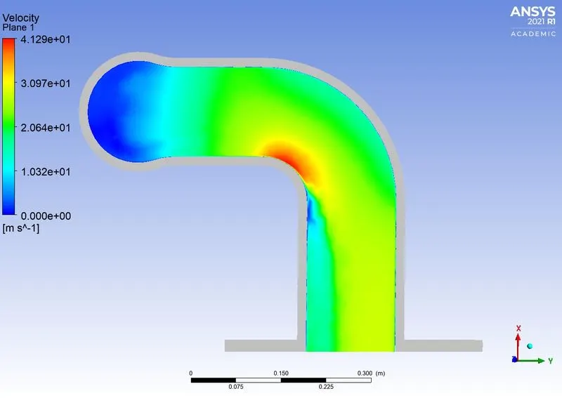- Fig 7 - Velocity contour

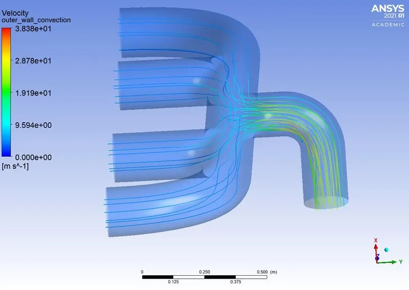- Fig 7.1 - Velocity contour

4. Conclusions:

• The numerical result of HTC has been verfied analytically with an error % of 3.1 - Hence the solution obtained is accurate.
• The reason for the distribution of velocity and temperature is - In the geometry, it can be observed that there are 4 inlets and only 1 outlet. So, according to conservation of mass, the entered mass must exit, which means that all the fluid from 4 different inlets to exit through one outlet, should have high velocity.
• High velocity means high kinetic energy, which further means higher temperature. So the regions outlined near the outlet region experience high velocity and temperature distribution.
• To verify the results, especially HTC value, various analytical relations can be use like Dittus-Boelter correlation, Sieder-Tate correlation and Whitaker correlation, etc.
• The conservation of mass along with above the mentioned co-relations are the factors which can be employed to determine the analytical values.
• While the details in the previous point correspond to analytical validation, there are some factors such as the initial conditions, boundary conditions, convergence criteria, meshing, solver selection, etc..which are important to be considered for numerical accuracy. These are the major factors on which the prediction accuracy depends on.

5. References

1. https://www.sciencedirect.com/topics/engineering/dittus-boelter-correlation
2. https://www.simscale.com/blog/2017/12/turbulence-cfd-analysis/#:~:text=LES%3A%20An%20average%20turbulence%20model,flows%20(unsteady%20for%20URANS).
3. https://skill-lync.com/knowledgebase/boundary-layer-y-plus-wall-functions-in-turbulent-flows-2
4. Applications of Mathematical Heat Transfer and Fluid Flow Models in Engineering and Medicine - Abram S. Dorfman.
5. Finite Analytic Method in Flows and Heat Transfer.