Multivariate Newton Rhapson Solver
Aim: To solve a system of non-linear equations using Multivariate Newton Rhapson method
1. Introduction:
To find the derivative of a single variable, Newton Rhapson method can be used. It can be either explicit or implicit. Explicit method tends to be a bit unstable, if proper time step size is not given. So, for the current problem implicit solver is chosen.
The implicit Newton Rhapson formula is given by:
`y^n = y^(n-1) + f.delt`, Where `y^n and y^(n-1)`are new and old values respectively. f is the function of which the derivative is to calculated and `delt`is the time step.
The above formula holds good for a single function. When multiple such functions are given as inputs, then Multivariate Newton Rhapson method is used. In the present case, 3 equations are given:
- `dy_1/dt = -0.04y_1 + 10^4*y_2*y_3`
- `dy_2/dt = 0.04y_1 - 10^4y_2y_3 - 3*10^7y_2^2`
- `dy_3/dt = 3*10^7y_2^2`
To convert the given equations into a root finding one, they are equated for RHS-LHS = 0.
`y_1^(n-1) + (-0.04y_1^n + 10^4y_2^ny_3^n)*delt - y_1^n = 0 rightarrow f_1`
`y_2^(n-1) + (0.04y_1 - 10^4y_2y_3 - 3*10^7y_2^2)*delt - y_2^n = 0 rightarrow f_2`
`y_3^(n-1) + (3*10^7y_2^2)* delt - y_3^n = 0 rightarrow f_3`
The formula used to calculate the new values of variables is:
- `y_(nw) = y_(guess) - alpha* (J^-1*F)`, where `y_(nw)`is the new values matrix - `y_(nw) = ((y1_(nw)), (y2_(nw)), (y3_(nw)))`, `y_(guess)`is the initial condition - `y_(guess) = ((y1_g),(y2_g),(y3_g))`
- Alpha is the under-relaxation factor.
- J is jacobian matrix and it contains the partial derivates of all functions wrt the 3 variables. `J = [[(delf_1)/dy_1, (delf_1)/dy_2, (delf_1)/dy_3],[(delf_2)/dy_1, (delf_2)/dy_2, (delf_2)/dy_3],[(delf_3)/dy_1, (delf_3)/dy_2, (delf_3)/dy_3]]`.
- The above matrix is an analytical matrix and in this problem, Jacobian is calculated numerically.
- F is the functions matrix - `F = ((f_1),(f_2),(f_3))`
While the normal Newton Rhapson method is used commonly to solve root finding problems, this can be used to solve chemical combustion equations, where each derivative can be considered as the rate of concentration change of reactants or products. And the variables can be considered as individual chemical species.
2. Coding approach:
- The required libraries such as matplotlib.pyplot, numpy and linalg are imported.
- 3 functions are created to solve the equations `f_1, f_2 and f_3`. Inputs are 3 new values, time step and an old value.
- Another function is created to solve jacobian numerically. This is done by forward differencing method. In the code, the parameter dy is the distance between two points y1 and y1+dy. As this distance tends to zero, the approximation improves.
- Initial conditions and time step array is defined.
- Matrices for old and guess values are created. These are initial matrices and contain only ones.
- Constants such error, tolerance and alpha are defined.
- A time step loop is created within which, a while loop calculates the new values of all the variables till the error term is less than tolerance.
- At the end of time step loop the new values are updated for next iteration.
- These updated values are stored in matrix to be plotted against time step.
3. Code:
import numpy as py
from numpy.linalg import inv
import matplotlib.pyplot as plt

def f1(y1, y2, y3, y1_old, dt):
	return (y1_old + (-0.04*y1 + pow(10,4)*y2*y3)*dt - y1)

def f2(y1, y2, y3, y2_old, dt):
	return (y2_old + (0.04*y1 - pow(10,4)*y2*y3 - (3*pow(10,7)*pow(y2,2)))*dt - y2)

def f3(y1, y2, y3, y3_old, dt):
	return (y3_old + (3*pow(10,7)*pow(y2,2))*dt - y3)

#Calculating the Jacobian matrix numerically
def jacobian(y1, y2, y3, y1_old, y2_old, y3_old, dt):

	J = py.ones((3,3))
	dy = 1e-5

	J[0,0] = (f1(y1+dy, y2, y3, y1_old, dt) - f1(y1, y2, y3, y1_old, dt))/dy
	J[0,1] = (f1(y1, y2+dy, y3, y1_old, dt) - f1(y1, y2, y3, y1_old, dt))/dy
	J[0,2] = (f1(y1, y2, y3+dy, y1_old, dt) - f1(y1, y2, y3, y1_old, dt))/dy

	J[1,0] = (f2(y1+dy, y2, y3, y2_old, dt) - f2(y1, y2, y3, y2_old, dt))/dy
	J[1,1] = (f2(y1, y2+dy, y3, y2_old, dt) - f2(y1, y2, y3, y2_old, dt))/dy
	J[1,2] = (f2(y1, y2, y3+dy, y2_old, dt) - f2(y1, y2, y3, y2_old, dt))/dy

	J[2,0] = (f3(y1+dy, y2, y3, y3_old, dt) - f3(y1, y2, y3, y3_old, dt))/dy
	J[2,1] = (f3(y1, y2+dy, y3, y3_old, dt) - f3(y1, y2, y3, y3_old, dt))/dy
	J[2,2] = (f3(y1, y2, y3+dy, y3_old, dt) - f3(y1, y2, y3, y3_old, dt))/dy

	return J

#Initial conditions
y1 = 1
y2 = 0
y3 = 0

#Time steps
start_time = 0
end_time = 600
dt = 0.1
nt = py.arange(start_time,end_time,dt)

#Defining matrices
y_old = py.ones((3,1))
y_guess = py.ones((3,1))

F = py.copy(y_guess)

y_final = py.ones((3,len(nt)))

iteration_time = 0
tol = 1e-7
alpha = 1

for a in range(1,len(nt)+1):

	y_old[0] = y1
	y_old[1] = y2
	y_old[2] = y3

	y_guess[0] = y1
	y_guess[1] = y2
	y_guess[2] = y3

	error = 9e9
	iterations = 0

	while error > tol:

		F[0] = f1(y_guess[0], y_guess[1], y_guess[2], y_old[0], dt)
		F[1] = f2(y_guess[0], y_guess[1], y_guess[2], y_old[1], dt)
		F[2] = f3(y_guess[0], y_guess[1], y_guess[2], y_old[2], dt)

		J = jacobian(y_guess[0], y_guess[0], y_guess[2], y_old[0], y_old[1], y_old[2], dt)

		y_new = y_guess - alpha*py.matmul(inv(J),F)
		error = py.max(py.abs(y_guess-y_new))

		y_guess = y_new

		log_message = 'iteration # = {0} y1 = {1} y2 = {2} y3 = {3}'.format(iter,y_new[0], y_new[1], y_new[2])
		#print(log_message)
		iterations = iterations +1

	y1 = y_new[0]
	y2 = y_new[1]
	y3 = y_new[2]

	y_final[0,iteration_time] = y_new[0]
	y_final[1,iteration_time] = y_new[1]
	y_final[2,iteration_time] = y_new[2]

	iteration_time = iteration_time + 1

print(iterations)
plt.plot(nt,y_final[0])
plt.plot(nt,y_final[1])
plt.plot(nt,y_final[2])
plt.xlabel('Total run time in seconds')
plt.ylabel('Final values of variables')
plt.legend(['Y1','Y2','Y3'])
plt.title('Variation of equation variables wrt time steps')
plt.show()
4. Results:
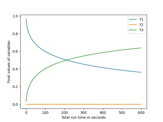
4.1 Time step size - 1s
Number of iterations to reach convergence - 1662
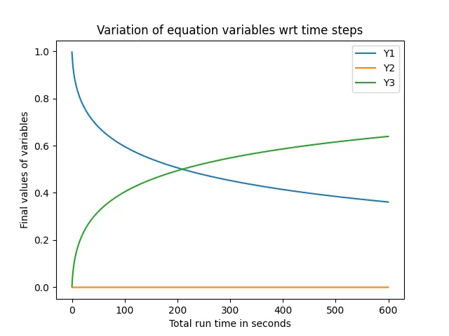
4.2 Time step size - 0.1s
Number of iterations to reach convergence - 168
4.3 Time step size - 0.05s
Number of iterations to reach convergence - 84
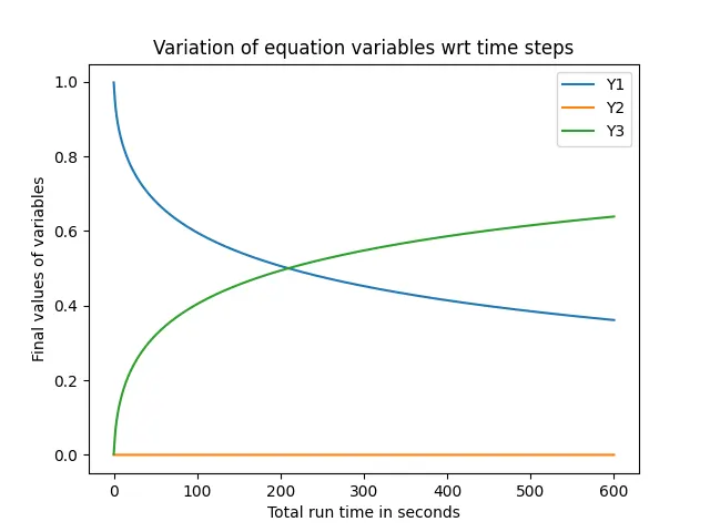
- From all the above images, it can be seen that the accuracy of results increase as the time step size is decreased. And the total run time is more for smaller time step, as the calculation has to run for longer time. For eg - for time step size of 1s, the run time is 600/1=600 seconds. And for time step size of 0.05s, the run time is 600/0.05 = 12000 seconds.
- As the time step size decreases, the number of iterations to reach convergence also decreases. Because the variation of results in every iteration is smaller, which provides accurate values.
- Also, as the implicit solver is used in this problem, the time step is assumed to be 1 initially and then it is decreased to 0.1 and 0.05. This is because the implicit solver is unconditionally stable. But for smaller time steps, it takes time to converge. And for this case, the ideal time step size would be 0.1.
5. References: