Solving the steady and unsteady 2D heat conduction problem using Matlab
Solving 2D Steady and Unsteady Heat Conduction equation using Matlab
Problem statement: To solve 2D Heat Conduction equation in steady state and unsteady state.
Theory:
Steady state analysis
The 2D heat conduction equation is steady state is given by: `(Delta^2T)/(Deltax^2)+(Delta^2T)/(Deltay^2)=0``
In the above equation, the temperature profile is obtained for the condition that temperature changes from one position to another provided the conditions at those 2 positions are different. It only depends on the space co-ordinates x,y.
The above equation after solving can be written as: `T(i,j) = (1/k)*[(T(i+1,j)+T(i-1,j))/(Deltax^2)+(T(i,j+1)+T(i,j-1))/(Deltay^2)]`, where `k = 2*(Deltax^2+Deltay^2)/((Deltax^2)*(Deltay^2))`;
- In the above equation T(i,j) is the present point or the point at which the equation needs to be solved. T(i+1,j) - Right side point, T(i-1,j) - Left side point, T(i,j+1) - Top point, T(i,j-1) - Bottom point.
- The equation is using neighbouring points to approximate the value at the current point. This improves accuracy. `Deltax and Deltay`are the distance between two different nodes in x and y direction respectively.
- To solve this equation is matlab, 3 approaches are considered. They are Jacobi method, Gauss Sedal method and Successive Over Relaxation (SOR) method. The advantage of using these methods is that, it is possible to compare the number of iterations taken by each method and identify an optimal method suitable for the purpose.
Matlab code is structured as follows:
- Domain conditions such as length, number of nodes in x and y directions are defined.
- Various constants such as dt, dx, dy SOR factor, error and tolerances are defined.
- Temperature matrix is defined for room temperature value.
- Boundary conditions are assigned.
- The solved equation is simplified.
- Loops are wrtitten for 3 methods and the results are plotted using contourf function.
Below Matlab code is for 2D steady state head conduction equation:
function Steady_State_Heat_Conduction_2D(method)

%Defining basic parameters
nx = 10; %Number of nodes in x direction.
ny = nx; %Number of nodes in y direction, which is equal to nodes in x direction.
L = 1; %Domain length.

x = linspace(0,L,nx);
dx = x(2)-x(1);

y = linspace(0,L,ny);
dy = dx;

%Temperature matrix. Assuming the domain temperature to be 300K.
T = 300*ones(nx,ny);

%SOR factor
w = 1.2;

%Boundary conditions
T(end,end) = 850; %Right Extreme bottom point temperature.
T(1,1) = 500; %Left extreme top point temperature.
T(1,end) = 700; %Right extreme top point temperature.
T(end,1) = 650; %Left extreme bottom point temperature.

T(1,2:end-1) = 600; %Top surface temperature.
T(2:end-1,1) = 400; %Left surface temperature.
T(end,2:end-1) = 900; %Bottom surface temperature.
T(2:end-1,end) = 800; %Right surface temperature.


%Storing the temperature matrix
T_old = T;

%Tolerance and error terms
error = 3e9;
tolerance = 1e-4;

%Simplifying the steady state equation
K = (2*(dx^2+dy^2))/((dx^2)*(dy^2));
Term_1 = 1/K;
Term_2 = Term_1*(1/dx^2);
Term_3 = Term_2;

%Loops to calculate the temperature values and plot them.

%Jacobi Method.
    if method == 1
        jacobi_iterations = 0;
        while error>tolerance
            for i = 2:nx-1
                for j = 2:ny-1

                    T(i,j) = Term_2*((T_old(i+1,j)+T_old(i-1,j))+(T_old(i,j+1)+T_old(i,j-1)));

                end
            end
            jacobi_iterations = 1+jacobi_iterations;
            error = max(abs(T_old(:)-T(:)));
            T_old = T;
        end
    [a, b] = contourf(x,y,T); %Creates a plot with color filled temperature representation.
    clabel(a,b); %Labels the temperature values on respective lines.
    set(gca, 'YDir','reverse') %Reverses the y-axis.
    colorbar;
    xlabel('Range of values in x direction')
    ylabel('Range of values in y direction')
    title(sprintf('2D Steady state heat conduction representation (Jacobi method) n Iterations = %d',jacobi_iterations));

    end


%Gauss Sedal Method.
        if method == 2
            gauss_iterations = 0;
            while error>tolerance
                for i = 2:nx-1
                    for j = 2:ny-1

                        T(i,j) = Term_2*((T_old(i+1,j)+T(i-1,j))+(T_old(i,j+1)+T(i,j-1))); %Temperature values are updated for the previous space co-ordinated in gauss sedal method.

                    end
                end
                gauss_iterations = 1+gauss_iterations;
                error = max(abs(T_old(:)-T(:)));
                T_old = T;
            end
        [a, b] = contourf(x,y,T);
        clabel(a,b);
        set(gca, 'YDir','reverse')
        colorbar;
        xlabel('Range of values in x direction')
        ylabel('Range of values in y direction')
        title(sprintf('2D Steady state heat conduction representation (Gauss Sedal method)n Iterations = %d',gauss_iterations));
        end


%Successive Over-relaxation Method.
        if method == 3
            sor_iterations = 0;
            while error>tolerance
                for i = 2:nx-1
                    for j = 2:ny-1

                        T(i,j) = (1-w)*T_old(i,j)+w*(Term_2*((T_old(i+1,j)+T(i-1,j))+(T_old(i,j+1)+T(i,j-1))));

                    end
                end
                sor_iterations = 1+sor_iterations;
                error = max(abs(T_old(:)-T(:)));
                T_old = T;
            end
        [a, b] = contourf(x,y,T);
        clabel(a,b);
        set(gca, 'YDir','reverse')
        colorbar;
        xlabel('Range of values in x direction')
        ylabel('Range of values in y direction')
        title(sprintf('2D Steady state heat conduction representation (SOR method)n Iterations = %d',sor_iterations));

        end
end
Results explanation:
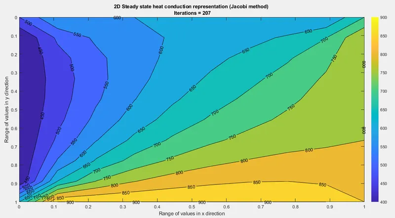
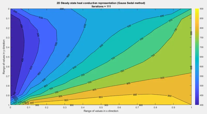
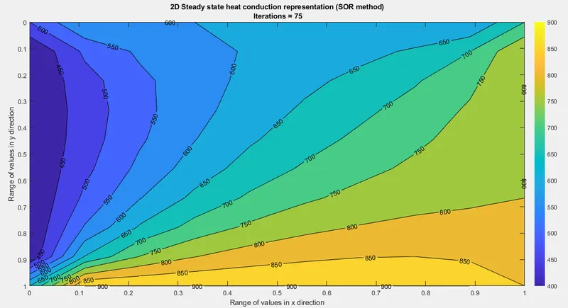
- It is evident from the above plots that the number of iterations have been decreasing as the methods are changed from Jacobi to SOR.
- The reason for this is - In Gauss Sedal method, the temperature values in the loop are changed with the calcualated values so the error converges to minimum as soon as possible and hence due to the same reason equation reaches steady state rapidly taking less computational time.
- Similarly in SOR method, a term called relaxation factor is introduced. This factor is introduced to affect the iterations. If the value of this factor is not correct, then the solution will be incomprehensible. So the right value is important for the solution to converge faster and take less iterations. In this problem, SOR factor is considered to be 1.2, which means that it is over-relaxed.
- The iteration trend observed is as follows : Jacobi>Gauss Sedal>SOR.
2D Unsteady state heat conduction equation solved using Explicit method
The equation for unsteady state analysis is: `(DT)/(Dt)=alpha*((Delta^2T)/(Deltax^2)+(Delta^2T)/(Deltay^2))`
Solved equation:`T(i,j) = T(i,j)+K1*(T(i+1,j)-2*T(i,j)+T(i-1,j))+K2*(T(i,j+1)-2*T(i,j)+T(i,j-1))`, where `K1 = alpha*(deltat)/(deltax^2) and K2 = alpha*(deltat)/(deltay^2)`
The only difference in this equation compared to steady state is the time derivative. Unsteady heat conduction is the substantial derivative of the temperature, which means that the temperature is changing at the current position with respect to time and its also changing due to the movement from one position to another where the influencing parameters have different values.
Here in explicit method, number of iterations depend on the time step and combines values of CFL numbers in both x and y directions. According to the standard condition for explicit method, CFL(x)+CFL(y)<=0.5. The values in matlab code for the time step and alpha is taken such that the above mentioned condition is satisfied.
The matlab code structure remains the same as steady state analysis, only addition is the time step loop, which is added to improve the convergence rate. Also, since the method is explicit, all the values in the RHS of the main equation are known. Hence, there was no need to use Jacobi, Gauss Sedal or SOR methods.
Matlab code:
function Unsteady_State_Heat_Conduction_2D_Explicit

%Defining basic parameters
nx = 10;
ny = nx;
L = 1;

x = linspace(0,L,nx);
dx = x(2)-x(1);

y = linspace(0,L,ny);
dy = dx;

%Temperature matrix. Assuming the domain temperature to be 300K.
T = 300*ones(nx,ny);

%Value of co-efficient alpha
a = 1.4;

%Boundary conditions
T(end,end) = 850; %Right Extreme bottom point temperature.
T(1,1) = 500; %Left extreme top point temperature.
T(1,end) = 700; %Right extreme top point temperature.
T(end,1) = 650; %Left extreme bottom point temperature.

T(1,2:end-1) = 600; %Top surface temperature.
T(2:end-1,1) = 400; %Left surface temperature.
T(end,2:end-1) = 900; %Bottom surface temperature.
T(2:end-1,end) = 800; %Right surface temperature.

%Storing the temperature matrix
T_old = T;

%Tolerance, error and time step terms
error = 3e9;
tolerance = 1e-4;
dt = 0.002; %Other values of dt will not yield proper results.

%Simplifying the unsteady state equation
CFL_1 = a*(dt/dx^2);
CFL_2 = a*(dt/dy^2);

%Time step
nt = 1;

%Loops to calculate the values of temperature at different space points and
%at different time steps.
    iterations = 0;
    for g = 1:nt
        while error>tolerance
            for i = 2:nx-1
                for j = 2:ny-1

                    term_1 = T_old(i-1,j)-2*T_old(i,j)+T_old(i+1,j);
                    term_2 = T_old(i,j+1)-2*T_old(i,j)+T_old(i,j-1);

                    T(i,j) = T_old(i,j)+(CFL_1*term_1)+(CFL_2*term_2);
                end
            end
            iterations = iterations+1; %Calculates the total iterations taken to reach convergence.
            error = max(abs(T_old(:)-T(:))); %Determines error in the old and present values of temperature.
            T_old = T;
        end
    end
[a, b] = contourf(x,y,T); %Plots temperature variation with color fill and the outputs are derived to represent temperature values.
clabel(a,b);
set(gca, 'YDir','reverse') %Reverses the y axis.
colorbar;
xlabel('Range of values in x direction')
ylabel('Range of values in y direction')
title(sprintf('2D heat conduction representation in transient state, Explicit method n CFL_x = %d,CFL_y=%d n Number of iterations = %d',CFL_1,CFL_2,iterations));

end
Result screenshot:
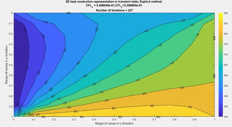
Explanation:
- Number of iterations taken to convergence is 227. This value is arrived at by trial and error method. The value of dt is imortant for the solution to conceive lesser iterations. Here the optimal value of dt is found to be 0.002. Any value other value will yield result, but iterations will go high.
- CFL number are also taken into account. CFL is a stability criterion usable when employing explicit method to solve the problem. This is kept below 0.5 as per the constraint for CFL criterion.
2D Unsteady State Heat Conduction Equation using Implicit method:
The equation for unsteady state analysis is: `T^(n+1)(i,j) = (T(i,j)+K1*(T(i+1,j)+T(i-1,j))^(n+1)+K2*(T(i,j+1)+T(i,j-1))^(n+1))/(1+2K1+2K2)`, where `K1 = alpha*(Deltat)/(Deltax^2) and K2 = alpha*(Deltat)/(Deltay^2)`
In this method, temperature are calculated for every time step. This means that as time changes the temperature also changes at its own position and when moved from one position to another. This is called implicit method.
The matlab code structure is similar to the previous one used in explicit method. The difference is the use of Jacobi, Gauss Sedal and SOR methods, since the variables used are almost unknown. Also, since the temperature values are evaluated for every time step, the temperature values are updated after every iteration to be used in the next iterations.
Matlab code:
function T_iteration = Unsteady_State_Heat_Conduction_2D_Implicit(iteration)

%Defining basic parameters
nx = 10;
ny = nx;
L = 1;

x = linspace(0,L,nx);
dx = x(2)-x(1);

y = linspace(0,L,ny);
dy = dx;

%Temperature matrix. Assuming the domain temperature to be 300K.
T = 300*ones(nx,ny);

%SOR factor
w = 1.2;

%Value of co-efficient alpha
a = 1.4;

%Boundary conditions
T(end,end) = 850; %Right Extreme bottom point temperature.
T(1,1) = 500; %Left extreme top point temperature.
T(1,end) = 700; %Right extreme top point temperature.
T(end,1) = 650; %Left extreme bottom point temperature.

T(1,2:end-1) = 600; %Top surface temperature.
T(2:end-1,1) = 400; %Left surface temperature.
T(end,2:end-1) = 900; %Bottom surface temperature.
T(2:end-1,end) = 800; %Right surface temperature.

%Storing the temperature matrix
T_old = T;
T_prev = T;

%Tolerance and error terms
error = 3e9;
tolerance = 1e-4;
dt = 0.002; %Time step value.

%Simplifying the unsteady state equation
CFL_x = a*(dt/dx^2); %Courant–Friedrichs–Lewy (CFL) number for x axis.
CFL_y = a*(dt/dy^2); %CFL number for y axis.
divisor = (1+2*CFL_x+2*CFL_y)^-1;

%Time step
nt = 1200;

%Loops to determine values of temperature in jacobi, gauss sedal and sor
%methods using time step and space loops.

%Jacobi method.
if iteration == 1
        jacobi_iterations = 0;
        tic;
        for n = 1:nt
            while error>tolerance
                    for i = 2:nx-1
                        for j = 2:ny-1

                            RL = (T_old(i+1,j)+T_old(i-1,j)); %Right and left points.
                            TB = (T_old(i,j+1)+T_old(i,j-1)); %Top and bottom points.
                            T(i,j) = divisor*(T_prev(i,j)+CFL_x*RL+CFL_y*TB);

                        end
                    end
                    error = max(abs(T_old(:)-T(:)));
                    T_old = T;
                    jacobi_iterations = 1+jacobi_iterations;
                    T_prev = T;
            end
            T_iteration = toc; %Storing time to indicate the computational time required to reach convergence.

        end
        [a, b] = contourf(x,y,T);
        clabel(a,b);
        set(gca, 'YDir','reverse')
        colorbar;
        xlabel('Range of values in x direction')
        ylabel('Range of values in y direction')
        title(sprintf('2D Unsteady state heat conduction representation in Jacobi method n Iterations = %d',jacobi_iterations));
end

%Gauss Sedal method.
if iteration == 2
        gauss_iterations = 0;
        tic;
        for n = 1:nt
            while error>tolerance
                    for i = 2:nx-1
                        for j = 2:ny-1

                            RL = (T_old(i+1,j)+T(i-1,j));
                            TB = (T_old(i,j+1)+T(i,j-1));
                            T(i,j) = divisor*(T_prev(i,j)+CFL_x*RL+CFL_y*TB);

                        end
                    end
                    error = max(abs(T_old(:)-T(:)));
                    T_old = T;
                    gauss_iterations = 1+gauss_iterations;
                    T_prev = T;
            end
            T_iteration = toc;
        end
        [a, b] = contourf(x,y,T);
        clabel(a,b);
        set(gca, 'YDir','reverse')
        colorbar;
        xlabel('Range of values in x direction')
        ylabel('Range of values in y direction')
        title(sprintf('2D Unsteady state heat conduction representation in Gauss Sedal method n Iterations = %d',gauss_iterations));
end

%Successive over-relaxation method.
if iteration == 3
        sor_iterations = 0;
        tic;
        for n = 1:nt
            while error>tolerance
                    for i = 2:nx-1
                        for j = 2:ny-1

                            RL = (T_old(i+1,j)+T(i-1,j));
                            TB = (T_old(i,j+1)+T(i,j-1));
                            T(i,j) = (1-w)*T_old(i,j)+divisor*w*(T_prev(i,j)+((CFL_x*RL+CFL_y*TB)));

                        end
                    end
                    error = max(abs(T_old(:)-T(:)));
                    T_old = T;
                    sor_iterations = 1+sor_iterations;
                    T_prev = T;
            end
        end
        T_iteration = toc;
        [a, b] = contourf(x,y,T);
        clabel(a,b);
        set(gca, 'YDir','reverse')
        colorbar;
        xlabel('Range of values in x direction')
        ylabel('Range of values in y direction')
        title(sprintf('2D Unsteady state heat conduction representation in SOR method n Iterations = %d',sor_iterations));
end
end
Screenshots:
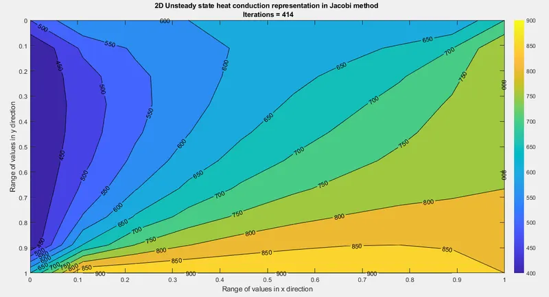
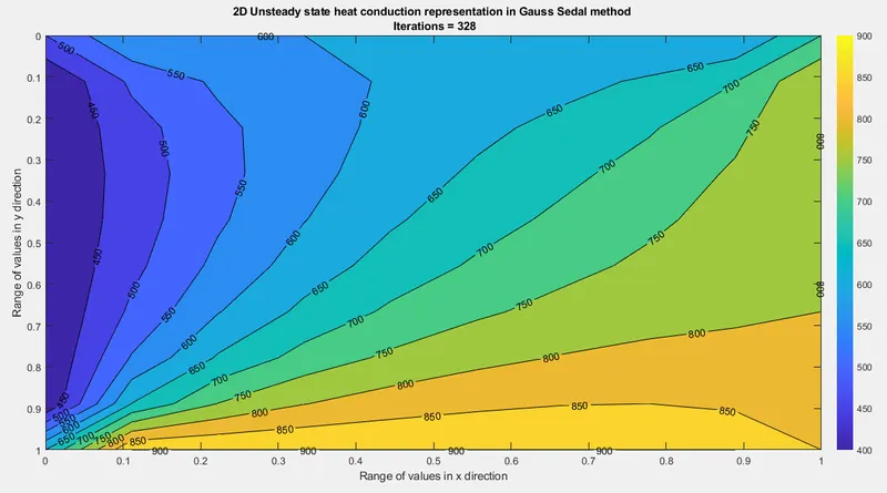
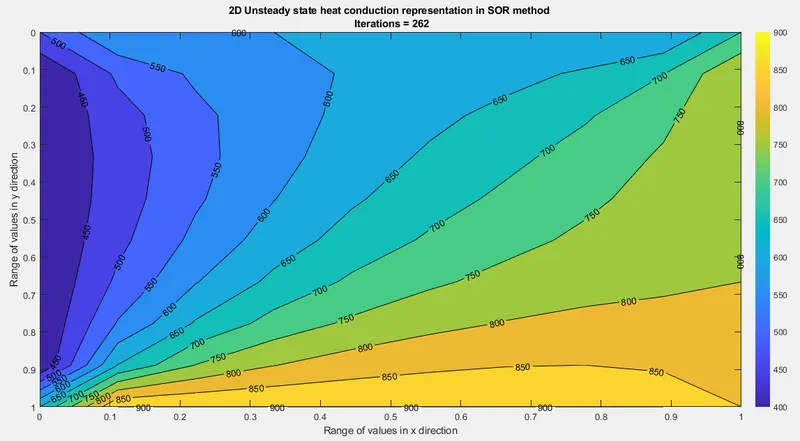
Explanation:
- The results fall in same category of steady state analysis. The number of iterations follow the trend: Jacobi>Gauss Sedal>SOR.
- The number of iterations are comparitively larger than steady state analysis due to addition of time step.
- The SOR factor is considered to be 1.2 here as well and the alpha value is kept same.
- The below table indicates the iterations taken by different methods in different approaches.
|
Steady state analysis |
Unsteady state analysis (Explicit method) |
Unsteady state analysis (Implicit method) |
|||||
|
Jacobi |
Gauss Sedal |
SOR |
Jacobi |
Gauss Sedal |
SOR |
||
|
Iterations |
207 |
111 |
75 |
227 |
414 |
328 |
262 |
It is clear from the above table that the explained trend is maintained throughout the results.