Simulation of Quasi 1D Super-sonic nozzle flow using MacCormack's technique
Aim: To perform the numerical simulations of isentropic flow through quasi 1-dimensional subsonic-supersonic nozzle flow in both conservation form and non-conservation form.
Theory:
A nozzle is a device which is used to alter or control the characteristics of a fluid as it exits from the outlet. Below is the image shown of a nozzle considered for this simulation. In the left hand side is the reservoir, which is assumed to have infinite area and hence the velocity of fluid will be theoritically zero in the reservoir. But practically, the velocity cannot be zero.
Other characteristics of fluid flow such as pressure and temperature are total values. The flow is subsonic in the convergent section, sonic at the throat and becomes supersonic throughout the divergent section. The flow is characterized to be isentropic, which means that there is no heat added to the fluid and no energy transformations occur due to friciton effects. The pressure, temperature, density, velocity and area are denoted respectively at convergent, throat and divergent sections as shown in the figure.
For the flow, area ratio is considered to be a function of x, meaning the variation of flow characteristics in the flow field is 1-dimensional and as mach number is a function of area ratio, it is in turn a function of x. Remaining characteristics such as pressure ratio, temperature ratio and density ratio are function of mach number.
To accelerate the flow at nozzle inlet, some form of input is required. This is the pressure ratio. It supplies the force required to accelerate the flow through the nozzle inlet. Also, for a given area ratio, pressure ratio is fixed and is treated as a boundary condition.
In the present case, the flow field variables are represented in terms of non-dimensional variables which vary between 0 and 1, such as `T = T/T_0, P = P/P_0, rho = rho/rho_0,V = V/a_0,etc.`
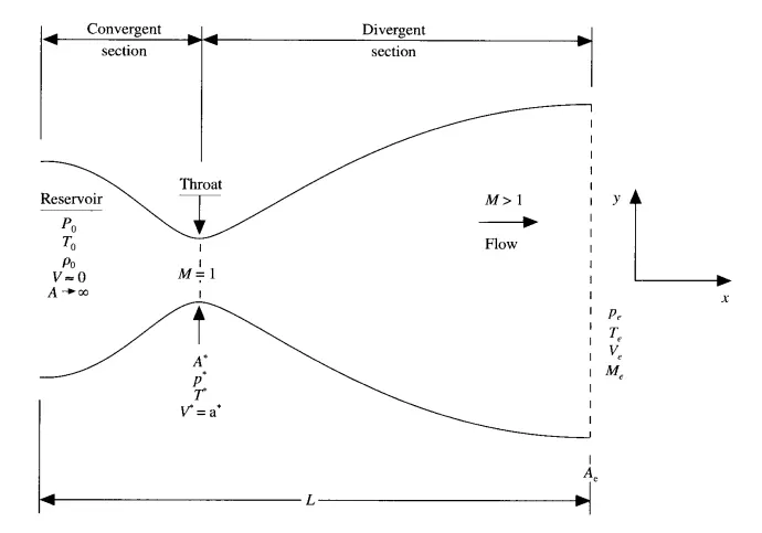
Basic governing equations for quasi 1-dimensional, steady, isentropic is given by:
Continuity equation:`rho_1*A_1*V_1 = rho_2*A_2*V_2`
Momentum equation: `p_1*A_1 + rho_1*V_1^2*A_1+(int_(A_1)^(A_2)P*dA = p_2*A_2 + rho_2*V_2^2*A_2`
Energy equation: `h_1+(V_1^2)/2 = h_2+(V_2^2)/2`
To simulate this numerical flow, MacCormak's method is used. This method is similar to lax wendroff's method, but is more simpler to solve.
- In Lax Wendroff's method, central differencing is used to get the second order accuracy and it also requires more time to derive the intermediate equations, which are required to solve different steps.
- In MacCormak's method, both forward and backward differencing are used to predictor and corrector steps respectively, which corressponds to second order accuracy. And the intermediate equations are not lengthy and also easy to derive, which is why it is used in this problem.
MacCormak's method:
This method basically involves two major steps - one is predictor step and the other is corrector step. Before understanding the steps, initially the governing equations are converted such that they are suitable time marching solution of quasi one-dimensional flow. After this step, the equations related to MacCormak's method are derived and finally, numerical solutions to those equations are determined.
Governing flow equations: When these are considered, two forms of governing equations can be derived and they are conservation and no-conservation forms. In conservation form, the assumption is that the control volume is fixed and the fluid moves in and out of the control volume. Here the control volume doesn't change its shape and size as the flow progresses.
In Non-conservation form, the control volume itself moves along with the fluid and hence it can change its shape and size with the flow. Practically both the forms are same, but numerically they are different.
-----------------------------------------------------------------------------------------------------------------------------------------------------------------------------------------------------------------------------------------
Non-conservative form:
Governing equations : Conitnuity equation - `(delrho)/(delt) = -rho*(delv)/(delx) - rho*v*(del(logA))/(delx) - v*(delrho)/(delx)`
Momentum equation - `(delv)/(delt) = -v*(delv)/(delx) - (1/gamma)[(delT)/(delx)+(T/rho)*(delrho)/(delx)]`
Energy equation - `(delT)/(delt) = -v*(delT)/(delx) - (gamma-1)*T*[(delv)/(delt)+v*(del(logA))/(delx)]`
For the above mentioned equations, predictor-corrector method is applied to arrive at solution after a specified value of time step dt.
Predictor method:
In the boundary conditions, the value of flow field variables are defined at time t. These variables are utilized while calculating the time derivatives explicitly. In this method, the value of time derivatives are calculated by using forward differencing approach, which uses the flow field variables at time step t. For eg:
`((delrho)/(delt))_i^t = -rho_i^t * (v_(i+1)^t-v_i^t)/(delx) - rho_i^t*v_i^t*((logA_(i+1)-logA_i))/(delx) - v_i^t*(rho_(i+1)^t-rho_i^t)/(delx)`
Similar to the above written equation, both momentum and energy equations are evaluated at time t. Then, the predicted values of flow field variables at t+dt is determined by using the expression, `rho_i^(t+dt) = rho_i^t + ((delrho)/(delt))_i^t*dt`.
Similarly, other predicted values are determined at the next time step. Below figure indicates the nodes distribution along x-axis inside the nozzle.
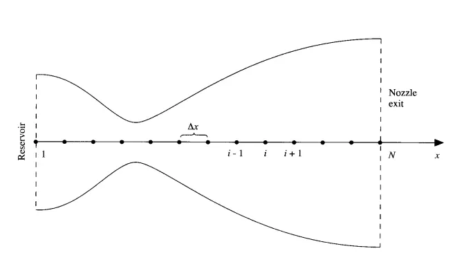
Corrector method:
In this method, backward differencing is used to determine the values at time step t+dt by using the predicted values of field variables. Eg:
`((delrho)/(delt))_i^(t+dt) = -rho_i^(t+dt) * (v_i^(t+dt)-v_(i-1)^(t+dt))/(delx) - rho_i^(t+dt)*v_i^(t+dt)*((logA_i-logA_(i-1)))/(delx) - v_i^(t+dt)*(rho_i^(t+dt)-rho_(i-1)^(t+dt))/(delx)`
Similar to the above equation, other time derivatives at time step t+dt is determined. After this, the values of time derivatives at time step t - determined in predictor step and time derivatives at time step t+dt - determined in corrector step are averaged such as, `((delrho)/(delt))_i^t = 0.5* [((delrho)/(delx))_i^t + ((delrho)/(delx))_i^(t+dt)]`.
Once the averaged value of time derivaties are determined, the actual flow field variables values are calculated by using the average time derivatives - `rho_i^(t+dt) = rho_i^t + ((delrho)/(delt))_(avg)*dt`. Similar to this other variables values are determined.
Time step:
Time step is determined by using, the formula - `dt = C*(delx)/(a+v)`. As per the stability criterion, the value of courant number(C) should be less 1 for hyperbolic partial differntial equations. For this problem, C is assumed to be 0.5. And the time step value is considered by calculating for all the variables values and then considering the minimum value out of them. Like this, the flow field variables after t+dt time, correspond to the same time which is favourable to compare with physical world results.
Boundary conditions:
Boundary conditions are important for the flow characteristics to turn out the way we want them to. As mentioned in theory part, to create a nozzle, area input is required and based on this area specific value of pressure is required for the flow. So there are two BCs and they are subsonic inflow and supersonic outflow.
Inflow: V1 = 2V2 - V3; Other variables such as density and temperature are fixed, as at the inlet a reservoir is assumed.
Outlet:`V_(N) = 2V_(N-1) - V_(N-2) ; rho_N = 2rho_(N-1)-rho_(N-2); T_N = 2T_(N-1)-T(N-2)`
Initial conditions:
Area: `A = 1+2.2*(x-1.5)^2 ; 0<=x<=3`
Density: `rho = 1-0.3146*x`
Temperature:`T = 1-0.2314*x`
Velocity:`V = (0.1+1.09x)*T^0.5`
-----------------------------------------------------------------------------------------------------------------------------------------------------------------------------------------------------------------------------------------
Conservative form:
Governing equations:
Continuity equation: `((del(rho*A))/(delt)) + ((del(rho*A*v))/(delx))=0`
Momentum equation: `((del(rho*A*v))/(delt)) + ((del(rho*A*v^2))/(delx))= -A*(delP)/(delx)`
Energy equation : `del[(rho*(e/(gamma-1)+(gamma/2)*v^2*A))) /(delt) + (del(rho*(e/(gamma-1)+(gamma/2)*v^2)*v*A+P*A*v))/(delx) = 0`
These equations can be represented in terms of generic form given by:
- Solution vectors, `U1 = rhoA; U2 = rhoAV; U3 = rho(e/(gamma-1)+(gamma/2)v^2)A`
- Flux vectors: `F1 = rhoAV; F2 = rhoAV^2+(1/gamma)pA; F3 = rho(e/(gamma-1)+(gamma/2)v^2)vA+pAv`
- Source term: `J2 = (1/gamma)*p*(delA)/(delx)`
By combining the above terms, governing equations are represented, which are - `(delU_1)/(delt) = -(delF_1)/(delx); (delU_2)/(delt) = -(delF_2)/(delx)+J2; (delU_3)/(delt) = -(delF_3)/(delx);`
The above equations are respectively continuity, momentum and energy equations.
MacCormak method is applied to the above mentioned equations similar to the non-conservation equations and the results are obtained.
Boundary conditions:
Inflow: `U_2(1) = 2U_2(2)-U_2(3)`
Outflow: `(U_1)_N=2(U_1)_(N-1)-(U_1)_(N-2); (U_2)_N=2(U_2)_(N-1)-(U_2)_(N-2); (U_3)_N=2(U_3)_(N-1)-(U_3)_(N-2);`
Initial conditions:
`rho = 1;T = 1; 0<=x<=0.5`
`rho = 1 - 0.366(x-0.5); T = 1 - 0.167(x-0.5); 0.5<=x<=1.5`
`rho = 0.634 - 0.3879(x-1.5); T = 0.833 - 0.3507(x-1.5); 1.5<=x<=3.5`
`v = 0.59/ (rhoA)`
-----------------------------------------------------------------------------------------------------------------------------------------------------------------------------------------------------------------------------------------
Matlab code: Non-conservation form
function [rho_th,T_th,p_th,M_th,m_dot] = oneD_nozzle_Non_conservative_method(N)
%Inputs
x = linspace(0,3,N);
dx = x(2)-x(1);
gamma = 1.4;

%Initial values
T_NC = 1-0.2314.*x; %Temperature
rho_NC = 1-0.3146.*x; %Density
v = (0.1+1.09.*x).*T_NC.^0.5; %Velcity
a = 1+2.2*(x-1.5).^2; %Area
m_dot = rho_NC.*a.*v; %Mass flow
throat = find(a==1); %Throat node value

%Time steps
nt = 1400;
C = 0.5;

for h = 1:nt

    rho_old = rho_NC;
    v_old = v;
    T_old = T_NC;

    %Predictor method
    for i = 2:N-1

        dv_dx(i) = (v(i+1)-v(i))/dx;
        drho_dx(i) = (rho_NC(i+1)-rho_NC(i))/dx;
        dlna_dx(i) = (log(a(i+1))-log(a(i)))/dx;
        dT_dx(i) = (T_NC(i+1)-T_NC(i))/dx;

        %Continuity equation
        drho_dt_p(i) = -rho_NC(i)*dv_dx(i) - rho_NC(i)*v(i)*dlna_dx(i) - v(i)*drho_dx(i);
        %Momentum equation
        dv_dt_p(i) = -v(i)*dv_dx(i)-(1/gamma)*(dT_dx(i)+(T_NC(i)/rho_NC(i))*drho_dx(i));
        %Energy equation
        dT_dt_p(i) = -v(i)*dT_dx(i)-(gamma-1)*T_NC(i)*(dv_dx(i)+v(i)*dlna_dx(i));

        dt(i) = C*(dx/((T_NC(i)^0.5)+v(i)));

        %updating the values
        v(i) = v(i)+dv_dt_p(i)*dt(i);
        rho_NC(i) = rho_NC(i)+drho_dt_p(i)*dt(i);
        T_NC(i) = T_NC(i)+dT_dt_p(i)*dt(i);
    end

    %Corrector method

    for j = 2:N-1

        dv_dx = (v(j)-v(j-1))/dx;
        drho_dx = (rho_NC(j)-rho_NC(j-1))/dx;
        dlna_dx = (log(a(j))-log(a(j-1)))/dx;
        dT_dx = (T_NC(j)-T_NC(j-1))/dx;

        %Continuity equation
        drho_dt_c(j) = -rho_NC(j)*dv_dx - rho_NC(j)*v(j)*dlna_dx - v(j)*drho_dx;
        %Momentum equation
        dv_dt_c(j) = -v(j)*dv_dx-(1/gamma)*(dT_dx+(T_NC(j)/rho_NC(j))*drho_dx);
        %Energy equation
        dT_dt_c(j) = -v(j)*dT_dx-(gamma-1)*T_NC(j)*(dv_dx+v(j)*dlna_dx);

        dt = min(C*(dx/((T_old(j)^0.5)+v_old(j))));

    end
    %Computing the average time derivatives
    drho_dt = 0.5.*(drho_dt_p + drho_dt_c);
    dv_dt = 0.5.*(dv_dt_p + dv_dt_c);
    dT_dt = 0.5.*(dT_dt_p + dT_dt_c);

    for w = 2:N-1
        %Updating the final values
        rho_NC(w) = rho_old(w)+drho_dt(w)*dt;
        T_NC(w) = T_old(w)+dT_dt(w)*dt;
        v(w) = v_old(w)+dv_dt(w)*dt;
    end

    p_NC = rho_NC.*T_NC;

    %Applying the boundary conditions
    %Inlet
    v(1) = 2*v(2)-v(3);

    %outlet
    rho_NC(N) = 2*rho_NC(N-1)-rho_NC(N-2);
    T_NC(N) = 2*T_NC(N-1)-T_NC(N-2);
    v(N) = 2*v(N-1)-v(N-2);
    p_NC(N) =  2*p_NC(N-1)-p_NC(N-2);

    m_dot = rho_NC.*v.*a;
    p_NC = rho_NC.*T_NC;
    M_NC = v./T_NC.^0.5;

    %Timewise variation of flow field variables at throat of the nozzle
    rho_th(h) = rho_NC(throat);
    T_th(h) = T_NC(throat);
    p_th(h) = p_NC(throat);
    M_th(h) = M_NC(throat);
    v_th(h) = v(throat);

    %Residuals
    Velocity_residual(h) = dv_dt(throat);
    Temperature_residual(h) = dT_dt(throat);
    Density_residual(h) = drho_dt(throat);

    figure(4)
    if h == 50
        plot(x,m_dot,'linewidth',1.25)
        hold on
        xlabel('Non-dimensional distance through the nozzle')
        ylabel('Non-dimensionl mass flow rate through the nozzle')
        title('Time dependent variation of mass flow inside the nozzle - Non-conservative form')
    elseif h == 100
        plot(x,m_dot,'linewidth',1.25)
    elseif h == 150
        plot(x,m_dot,'linewidth',1.25)
    elseif h == 200
        plot(x,m_dot,'linewidth',1.25)
    elseif h == 500
        plot(x,m_dot,'linewidth',1.25)
    elseif h == 700
        plot(x,m_dot,'linewidth',1.25)
        legend('50dt','100dt','150dt','200dt','500dt','700dt','linewidth',1.25)
    end

end
    %Plots
    figure(5)
    tiledlayout(4,1)

    %First plot
    nexttile
    plot(x,M_NC)
    title({['Non conservative form'],['Steady state distribution of Velocity inside the nozzle']})
    ylabel('Mach number')

    %Second plot
    nexttile
    plot(x,p_NC)
    title('Steady state distribution of Pressure inside the nozzle')
    ylabel('Pressure ratio')

    %Third plot
    nexttile
    plot(x,rho_NC)
    title('Steady state distribution of Density inside the nozzle')
    ylabel('Density ratio')

    %Fourth plot
    nexttile
    plot(x,T_NC)
    title('Steady state distribution of temperature inside the nozzle')
    xlabel('Non dimensional distance through nozzle')
    ylabel('Temperature ratio')

    time = linspace(1,nt,nt);

    figure(6)
    hold on
    plot(time,Velocity_residual,'linewidth',1.2)
    title('Time wise variations of absolute values of time derivatives -  Non-conservative form')
    xlabel('Number of time steps')
    ylabel('Residual')

    plot(time,Temperature_residual,'linewidth',1.3)

    plot(time,Density_residual,'linewidth',1.3)
    legend('Velocity residuals','Temperature residuals','linewidth',1)


end
Plots:
Steady state distribution of primitive variables inside the nozzle:
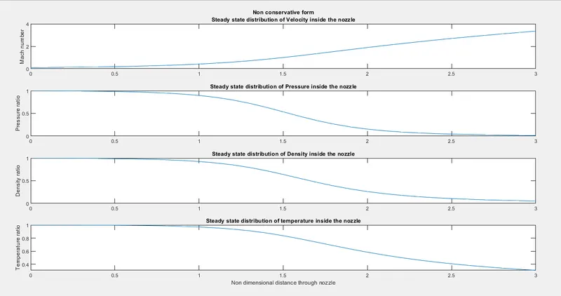
- From the above plot, it can be clearly observed that the primitive variables vary realistically, that is as they approach mach number 1, due to the convergent subsonic nozzle section, temperature, pressure, density increases and as the flow moves from the nozzle throat, after which mach number increases beyond 1, these values decrease with time and reach steady state after a specific amount of time.
Variation of Mass flow rate distribution inside the nozzle at different time steps during the time-marching process:
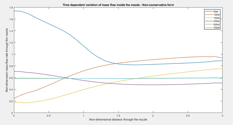
- The above figure indicates the variation of mass flow rate at the throat section of nozzle. It can be inferred that, the mass flow varies with time till around 400 time steps, after which it reaches steady state and there will be no variation in the mass flow. Here mass flow is considered to be a function of internal grid points or distance through the nozzle. This means after nearly 300 to 400 time steps `rhoVA =`constant.
Residuals plot:
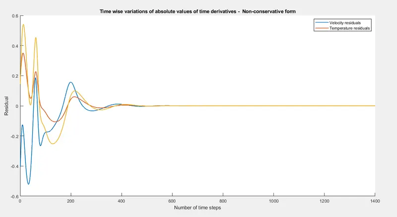
- The above residual plot indicates that the time derivatives oscillate initially and these osciallations are attributed to the unsteady compression and expansion in the nozzle. Also after nearly 500 time steps, oscillations converge and the solution reaches steady state, though the values never converge to zero. They will be extremely minute in the orders of 1e-7.
-----------------------------------------------------------------------------------------------------------------------------------------------------------------------------------------------------------------------------------------
Conservation form:
function [rho_th_C,T_th_C,v_C,P_th_C,U2,M_th_C,rho_gc,T_gc,M_gc,P_gc] = OneD_Nozzle_Conservative_method(N)

%Inputs
x = linspace(0,3,N);
dx = x(2)-x(1);
gamma = 1.4;
nt = 1400; %Time steps
C = 0.5;%Courant number

%Initial values for density and temperature
for i = 1:N

    if x(i)>=0 && x(i)<=0.5
        rho_C(i) = 1; T_C(i) = 1;

    elseif x(i)>=0.5 && x(i)<=1.5
        rho_C(i) = 1 - 0.366*(x(i) - 0.5);
        T_C(i) = 1 - 0.167*(x(i) - 0.5);

    elseif x(i)>=1.5 && x(i)<=3
        rho_C(i) = 0.634 - 0.3879*(x(i) - 1.5);
        T_C(i) = 0.833 - 0.3507*(x(i) - 1.5);

    end
end
%Initial values for area and velocity
a = 1 + 2.2*(x - 1.5).^2; %Area
v_C = 0.59./(rho_C.*a); %Velocity
throat = find(a==1) %Throat node value

for k = 1:nt

    %Dependent variables calculated in pure form
    U1 = rho_C.*a;
    U2 = rho_C.*a.*v_C;
    U3 = rho_C.*((T_C/(gamma-1)) + (gamma*(v_C.^2)/2)).*a;

    F1 = U2;
    F2 = (U2.^2./U1) + ((gamma-1)/gamma) * (U3-((0.5*gamma) * (U2.^2./U1)));
    F3 = (gamma*((U2.*U3)./U1)) - ((gamma*(gamma-1)/2) * (U2.^3./U1.^2));

    %Keeping the old values
    U1_old = U1;
    U2_old = U2;
    U3_old = U3;

    %Predictor method
    for m = 2:N-1

        da_dx = (a(m+1) - a(m))/dx;
        J2(m) = (rho_C(m) * T_C(m) * da_dx)/gamma;

        %Using forward differencing to calcuate the value of flux terms.

        dU1_dt_p(m) = -(F1(m+1) - F1(m))/dx; %Continuity equation

        dU2_dt_p(m) = -(F2(m+1) - F2(m))/dx+J2(m); %Momentum equation

        dU3_dt_p(m) = -(F3(m+1) - F3(m))/dx; %Energy equation

        %Value of dt
        dt = min(C * (dx/((T_C(m)^0.5)+v_C(m))));

        %Predicted values of dependent varibles
        U1(m) = U1(m) + dU1_dt_p(m) * dt;
        U2(m) = U2(m) + dU2_dt_p(m) * dt;
        U3(m) = U3(m) + dU3_dt_p(m) * dt;

        %Predicted values of primitive variables
        rho_C(m) = U1(m)/a(m);
        T_C(m) = (gamma-1) * ((U3(m)/U1(m)) - (gamma*0.5) * (U2(m)/U1(m))^2);

        %Predicted values of flux variables
        F1(m) = U2(m);
        F2(m) = (U2(m)^2/U1(m)) + ((gamma-1)/gamma) * (U3(m)-((0.5*gamma) * (U2(m)^2/U1(m))));
        F3(m) = (gamma*((U2(m)*U3(m))/U1(m))) - ((gamma*(gamma-1)/2) * (U2(m)^3/U1(m)^2));

    end

%Corrector method
    for p = 2:N-1

        da_dx = (a(p) - a(p-1))/dx;
        J2(p) = (rho_C(p) * T_C(p) * da_dx)/gamma;

        %Using backward differencing to calcuate the value of flux terms.

        dU1_dt_c(p) = -((F1(p) - F1(p-1))/dx); %Continuity equation

        dU2_dt_c(p) = -((F2(p) - F2(p-1))/dx)+J2(p); %Momentum equation

        dU3_dt_c(p) = -((F3(p) - F3(p-1))/dx); %Energy equation

        %Averaging the time derivatives
        dU1_dt(p) = 0.5 * (dU1_dt_p(p) + dU1_dt_c(p));
        dU2_dt(p) = 0.5 * (dU2_dt_p(p) + dU2_dt_c(p));
        dU3_dt(p) = 0.5 * (dU3_dt_p(p) + dU3_dt_c(p));

        %Final corrected values
        U1(p) = U1_old(p) + dU1_dt(p) * dt;
        U2(p) = U2_old(p) + dU2_dt(p) * dt;
        U3(p) = U3_old(p) + dU3_dt(p) * dt;
    end

        %Applying the boundary conditions
        %Inflow
        U1(1) = rho_C(1)*a(1);
        U2(1) = 2*U2(2) - U2(3);
        U3(1) = U1(1)*(T_C(1)/(gamma-1)+gamma/2*(U2(1)/U1(1))^2);

        %Outflow
        U1(N) = 2*U1(N-1) - U1(N-2);
        U2(N) = 2*U2(N-1) - U2(N-2);
        U3(N) = 2*U3(N-1) - U3(N-2);

        %Extracting the value of primitive variables from flow field
        %variables
        rho_C = U1./a;
        v_C = U2./U1;
        T_C = (gamma-1)*((U3./U1) - gamma*0.5*v_C.^2);
        P_C = rho_C.*T_C;
        M_C = v_C./T_C.^0.5;

        %Timewise variation of flow field variables at the nozzle throat
        rho_th_C(k) = rho_C(throat);
        T_th_C(k) = T_C(throat);
        P_th_C(k) = P_C(throat);
        M_th_C(k) = M_C(throat);

        %residuals
        velocity_res1(k) = dU1_dt(throat);
        velocity_res2(k) = dU2_dt(throat);
        velocity_res3(k) = dU3_dt(throat);

        figure(1)
        %mass flow rate variation as a function of time steps
        hold on
            if k == 50
                plot(x,U2,'b','linewidth',1.5)
                title('Time wise variation of Mass flow inside the nozzle - Conservative form')
            elseif k == 100
                plot(x,U2,'g','linewidth',1.5)
            elseif k == 150
                plot(x,U2,'m','linewidth',1.5)
            elseif k == 200
                plot(x,U2,'c','linewidth',1.5)
            elseif k == 700
                plot(x,U2,'r','linewidth',1.5)
                legend('50dt','100dt','150dt','200dt','700dt','linewidth',1,'Location','North')
                xlabel('Non-dimensional distance through nozzle')
                ylabel('Non-dimensional mass flow through nozzle')
            end

end
    %Plots
    figure(2)
    tiledlayout(4,1)

    %First plot
    nexttile
    plot(x,M_C)
    title({['Conservative form'],['Steady state distribution of Velocity inside the nozzle']})
    ylabel('Velocity ratio')

    %Second plot
    nexttile
    plot(x,P_C)
    title('Steady state distribution of Pressure inside the nozzle')
    ylabel('Pressure ratio')

    %Third plot
    nexttile
    plot(x,rho_C)
    title('Steady state distribution of Density inside the nozzle')
    ylabel('Density ratio')

    %Fourth plot
    nexttile
    plot(x,T_C)
    title('Steady state distribution of temperature inside the nozzle')
    xlabel('Non dimensional distance through nozzle')
    ylabel('Temperature ratio')

    time = linspace(1,nt,nt);

    figure(3)
    hold on
    plot(time,velocity_res1,'linewidth',1.25)
    title('Time wise variations of absolute values of time derivatives - Conservative form')
    xlabel('Number of time steps')
    ylabel('Residual')

    plot(time,velocity_res2,'linewidth',1.25)

    plot(time,velocity_res3,'linewidth',1.25)
    legend('U1-residuals','U2-residuals','U3-residuals','linewidth',1)

    %for grid dependency test
    rho_gc = rho_C(throat);
    T_gc = T_C(throat);
    M_gc = M_C(throat);
    P_gc = P_C(throat);
end
Plots:
Steady-state distribution of primitive variables inside the nozzle
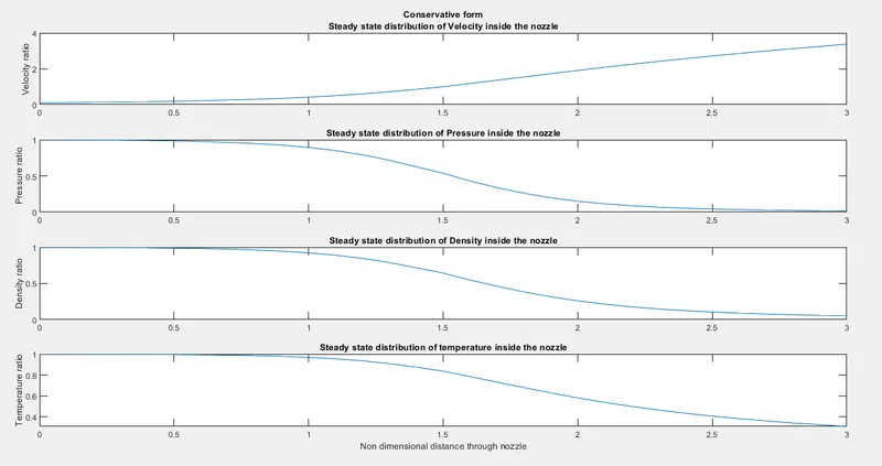
- Similar to non-conservative method, the above figure indicates that the variation is realistic and agrees with the numerical results.
Variation of Mass flow rate distribution inside the nozzle at different time steps during the time-marching process:
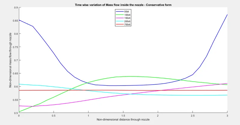
- This indicates that even conservative form of mass flow converges near 500 time steps.
Residual plot:
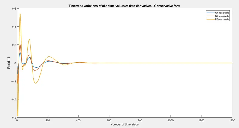
- A similar conclusion can be inferred for residuals as in the case of non-conservative form.
Main code which can be run to obtain both results of conservative form and non-conservative form:
%Inputs
N = 31;
x = linspace(0,3,N);
dx = x(2)-x(1);
gamma = 1.4;
nt = 1400; %Time steps

tic
[rho_th_C,T_th_C,v_C,P_th_C,U2,M_th_C] = OneD_Nozzle_Conservative_method(31);
end_time_c = toc

tic
[rho_th,T_th,p_th,M_th,m_dot] = oneD_nozzle_Non_conservative_method(31);
end_time_NC = toc

time = linspace(1,nt,nt)
figure(7)
hold on
tiledlayout(4,1)

nexttile
plot(time,rho_th_C,time,rho_th,'linewidth',1.2)
title('Time wise variation of primitive variables inside the nozzle')
ylabel('Density ratio')
legend('Conservative form','Non-conservative form','linewidth',1)

nexttile
plot(time,T_th_C,time,T_th,'linewidth',1.2)
ylabel('Temperature ratio')

nexttile
plot(time,P_th_C,time,p_th,'linewidth',1.2)
ylabel('Pressure ratio')

nexttile
plot(time,M_th_C,time,M_th,'linewidth',1.2)
xlabel('Number of time steps')
ylabel('Mach number')

for q = 1:N
    Analytical_solution(q) = 0.579;
end

figure(8)
hold on
plot(x,U2,x,m_dot,x,Analytical_solution,'linewidth',1.5)
title('Steady state flow variations of both Non-conservative and conservative forms of governing equations')
xlabel('Non-dimensional distance through nozzle')
ylabel('Non-dimensional mass flow through the nozzle')
legend('Conservative form','Non-conservative form','Analytical solution','linewidth',1,'Location','North')
Combined plots:
Time-wise variation of the primitive variables
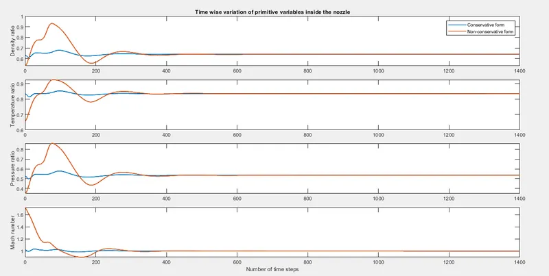
- Here, the variation of primitive variables is higher in case of non-conservative form. This is because initially, the flow field variables are driven by a stronger potential. As time increases this strong potential decreases its effect and hence the variables reach convergence.
- Since in conservative form, fluid moves in and out of the control volume, the strong potential is comparitively less and hence lesser variations.
Comparison of Normalized mass flow rate distributions of both forms
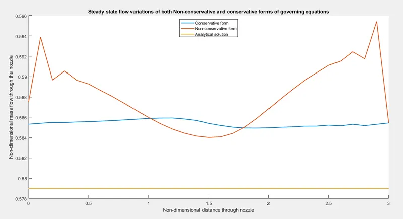
- This figure indicates the closeness of numerical solutions (of mass flow rate) to the exact analytical solution. It can be inferred that the conservative form is more accurate.
- This is because, the mass flow itself is a dependent variable in conservative form and mass flow in non-conservative form is obtained by primitive variables.
-----------------------------------------------------------------------------------------------------------------------------------------------------------------------------------------------------------------------------------------
Grid-dependency test:
|
Sl.no |
Type of solution |
Number of nodes |
Primitive variables |
%Deviation from exact value (only density is considered) |
|||
|
Density |
Temperature |
Pressure |
Mach number |
||||
|
1 |
Exact |
31 |
0.634 |
0.833 |
0.528 |
1 |
0 |
|
2 |
Non-conservative |
31 |
0.6390 |
0.8366 |
0.5346 |
0.9992 |
1.007 |
|
3 |
Conservative |
31 |
0.6429 |
0.8361 |
0.5376 |
0.9958 |
1.014 |
|
4 |
Non-conservative |
61 |
0.6377 |
0.8354 |
0.5327 |
0.9997 |
1.005 |
|
5 |
Conservative |
61 |
0.6375 |
0.8348 |
0.5322 |
1.0006 |
1.005 |
|
6 |
Non-conservative |
121 |
0.6308 |
0.8318 |
0.5247 |
0.9886 |
-1.005 |
|
7 |
Conservative |
121 |
0.6361 |
0.8344 |
0.5308 |
0.9980 |
1.003 |
- It can be inferred from the table that, even after increasing the number of grid points or refining the mesh, numerical solutions doesn't seem to change much with respect to the exact solution.
- Both conservation and non-conservation forms are very close to the exact solution and increasing the grid points also yield the same effects.
- The deviation is very less. (only density deviation is shown in the table, although the deviations of other variables also falls in the similar range)
- This means no at 31 grid points, grid independency is achieved.
Conclusion:
- Practically both conservation and non-conservation forms are the same and the only difference is in the numerial procedures.
- When mass conservation is considerd, conservation form is better and if residuals are considered non-conservation form is better as the value of residuals is very less.
- In terms of solving, non-conservation form is a little more easy to solve because in conservation form flux variables, solution variables have to be first calculated and then the equations need to be applied.
- There are no differences in terms of stability or exactness of solutions between conservation and non-conservation forms.
References:
- Computational fluid dynamics: The basics with applications