Prandtl Meyer Shock problem

Aim: To simulate Prandtl-Meyer shock using CONVERGE CFD

1. Introduction:

In Prandtl-Meyer shock problem, a supersonic flow is expands around a sharp corner. The shrap corner can be seen in the geometry just after the inlet.

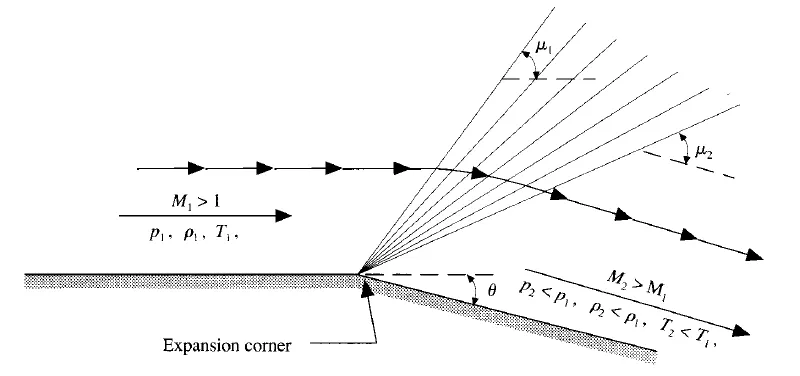Source: CFD: The basics with applications - John.D.Anderson

Once the shock reaches the sharp corner, expansion starts - expansion wave. Under this expansion wave, infinite number of weak mach waves get generated. The flow through this expansion wave is isentropic. Flow conditions starting from inlet such as pressure, temperature, density increase and reach their maximum values when they form the expansion wave.

In the region past the expansion wave, flow properties decrease in magnitude, but vary smoothly. The discontinuity in flow field variables happen only at the sharp corner.

Shock waves

Conisder an aircraft moving below the speed of sound. The air molecules right in front of the aircraft are compressed and this compression results in pressure waves. The pressure waves generated here are smooth and they are generated in a circular pattern. None of the pressure waves interfere (constructive or destructive) with each other and hence there will be no abrupt change in pressure, temperature, density, etc.

Now, consider an aircraft moving faster than the speed of sound. The pressure waves formed due to compression of air molecules are behind the aircraft and they take the form of a cone. The angle of this cone reduces as the speed of aircraft increases further.

The circular pressure waves at each point in front of the aircraft interfere constructively (crust to crust) with each other and create a high pressure region, which is immediately followed by a low pressure region. This high pressure conical region is known as a Shock. This shock traverses in the air medium in the form of waves. When these waves hit the ground, sonic boom is heard.

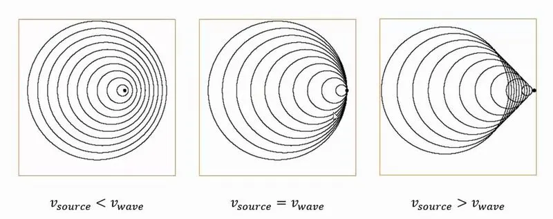
Shock waves are generated in diverse situations such as when a bullet is fired, when an aircraft breaks the sound barrier, after whipping a rope in air, etc.

1.1 Governing equations

The flow is 2D, inviscid and represented in conservation form. Governing Euler equations are given by:

• Continuity - `(delrho)/(delt) + nabla.(rhoV) = 0`
• Momentum -
  
  • X - component - `rho. (Du)/(Dt) = -(delP)/(delx)`
  • Y - component - `rho. (Dv)/(Dt) = -(delP)/(dely)`
  • Z - component - `rho. (Dw)/(Dt) = -(delP)/(delz)`
• Energy - `del/(delt)[rho(e + V^2/2)] + nabla[rho(e + V^2/2)V'] = rho*q - (del(uP))/(delx) - (del(vP))/(dely) - (del(wP))/(delz)`

Body force is not considered and V' is energy equation is the volume.

Conservation form of equations are used as they capture shocks better than non-conservation form of equations.

2. Solution Approach:

• Import the geometry to Converge studio.
• Scale to appropriate dimensions.
• Define inlet, outlet, 2D and wall boundaries.
• Check for errors.
• Select time based application.
• Consider gas-type simulation with air as predefined mixture in materials.
• Select Steady-state solver for the simulation - set number of cycles - 15000.
• Define a volumetric region containing air with inlet velocity.
• Define boundary conditions (Dirichlet at inlet and Neumann at outlet).
• Set Steady state monitor parameters.
• Select RNG K - epsilon turbulence model.
• Define grid size - 5mm and define Adaptive Mesh refinement based on Temperature curve.
• Export input files to a folder and run the simulation on Cygwin command prompt.
• Convert the post.h files to paraview format and post process the results.

3. Pre-processing:

3.1 Geometry

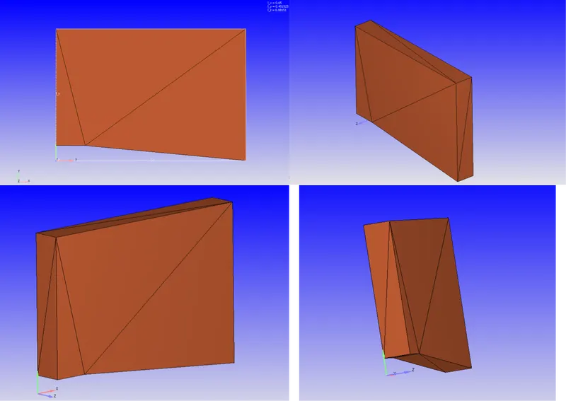
• The dimensions of geometry are - 0.65m*0.45m*0.081m.

3.2 Mesh

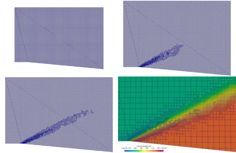
• The above images shows the mesh refinement structure. Base mesh size is 5mm.
• Adaptive mesh refinement is defined based on the difference in temperature curves. For this case, the difference value considered is 0.05k.
• AMR for the value 0.05k does not cover the entire shock region and it can be seen in the bottom left image. This image represents flow in its last cycle.
• Number of embedd layers considered for this is 3. If there is region in the flow field with difference value less than 0.05k, then AMR keeps refining it with 3 embedd layers, until a region is encountered with difference value more than 0.05k.
• The bottom right image shows the shock formation at the end of simulation with mesh refinement.

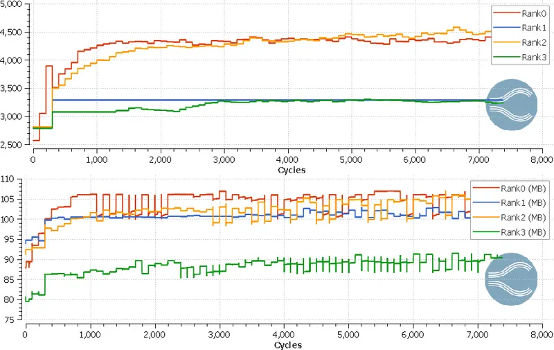
• Total number of cycles for this case are observed to be a little more than 15000.
• Total memory used during the simulation - around 520MB.

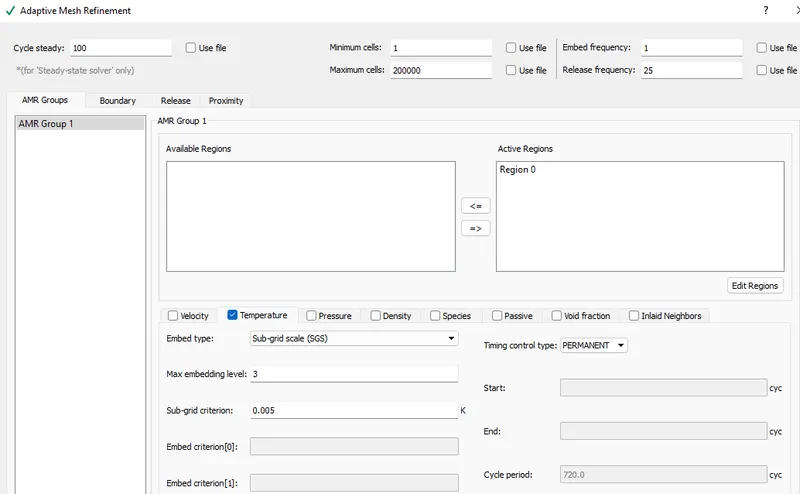
• The above image shows the details of AMR.

4. Solver:

Solver set-up details
Steady state monitor details		Simulation time parameters		Solver parameters		Boundary conditions
Min number of cycles to be executed	7000	Total number of cycles	15000	Solver scheme	PISO	Inlet	Velocity - 678m/s and Pressure - 101325pa
Monitor start delay in cycles	200	Min time step	1e-9s	Solver type	Pressure - based	Outlet	Neumann BC
Sample size, cycles	100	Max time step	1s	Equation solver type	SOR	Front and Back walls	2D
Relative tolerance	0.01	Max convection CFL limit	0.5	SOR relaxation	1	Top and Bottom walls	Wall BC - Slip

• Tubulence model is not used for this simulation as the fluid is considered to be inviscid.

4.1 Boundary conditions

In any fluid flow problem, if we want the fluid to behave in a particular way, then certain conditions have to be imposed. These conditions could define the convergence rate, accurately predict the real world physics, etc.

In this study, supersonic flow needs to be imposed at the inlet to derive proper outputs. This is done by using Dirichlet BC. This BC allows to define variable values. So, conditions such as velocity, temperature and pressure are defined. Generally, for problems involving shocks, Dirichlet BC is used.

Neumann BC is defined at the outle - zero gradients for velocity, temperature and pressure. Using this BC, derivative of a variable can be defined. When values for certain variables needs to be imposed in terms of gradients, this BC can be used.

5. Post processing:

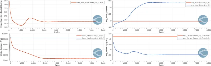
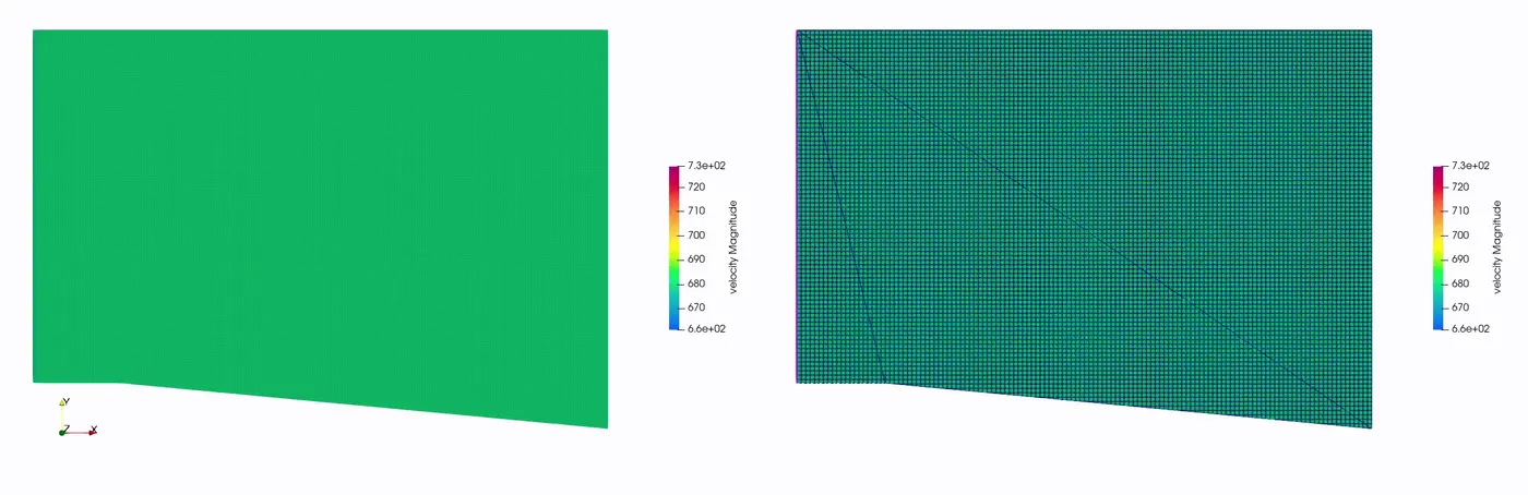
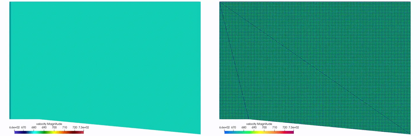
• Sharp changes seen in the below images can be attributed to the time of formation of the expansion wave at the sharp corner.
• The Mach number increases and stays constant throughtout flow at 2.14M.

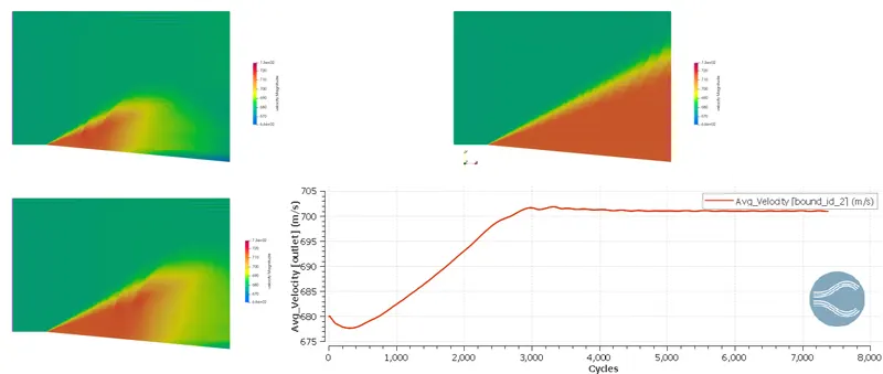
• Formation of expansion wave in series can be observed in the below images. The contour indicates velocity distribution.
• A number of weak mach waves (weak because low in pressure, temperature and density, but high in velocity) can be seen in the top right image.
• Line plot indicates the average velocity of 2.14M is reached around 3000 cycles in the simulation, after which it remains constant.

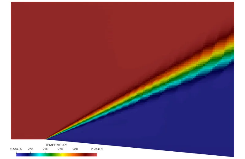
• The below image shows the temperature distribution. Temperature can be seen to reduce right after the expansion wave.
• Blue zone indicates the weak Mach wave region.

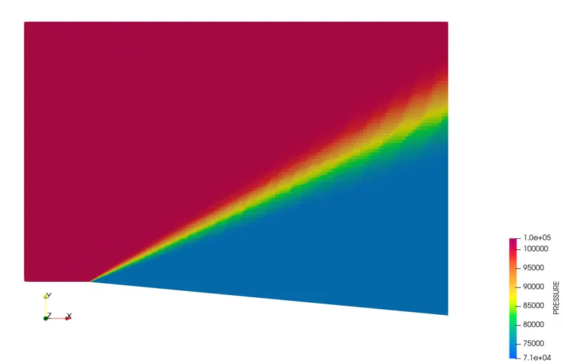
• Pressure distribution is also similar to temperature distribution. Pressure decreases after the expanion wave and remains constant.

5.1 Effect of SGS - Sub-Grid-Scale temperature value on cell count and shock location

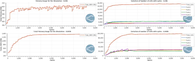
• To refine areas near the expansion wave, AMR is used. In AMR, sub-grid type of embedding is used. The sub-grid criterion is the difference in temperature of different curves. Before this section, all the results presented are for Sub-grid criterion 0.05K.
• In the above image, the line plots for cell count and memory usage are compared between sub-grid criterion 0.05K and 0.005K.
• The total memory used during the simulation triples over a decrease of grid-criterion factor by 10.
• In this SGS type of embedding, if the solver detects temperature curves whose difference is below the set criterion, it refines the area until the difference expeeds the criterion. This is why the number of cells and memory increase by many folds when the criterion is decreased by a factor of 10.
• The number of cells for 0.05K criterion is around 15,000 and for 0.005K criterion it is around 100,000.

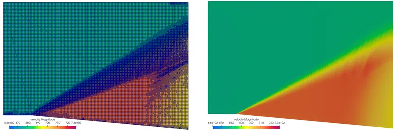
• The above images shows the velocity contours with mesh refinement on the left and without mesh on the right for 0.005K criterion.

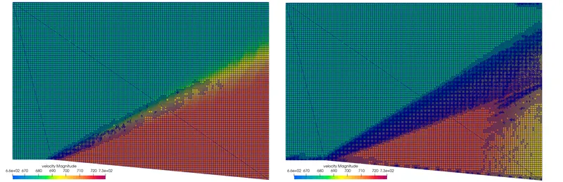
• The difference in mesh refinement for criterions 0.05K and 0.005K can be seen in the above image. Left image indicates the velocity contour with mesh refinement for 0.05K and the right image is for velocity contour with mesh refinement for 0.005K.

5.3 Simulation of Expansion wave

For 0.05K SGS criterion

For 0.005K SGS criterion

6. Resources:

1. https://www.physicsclassroom.com/class/sound/Lesson-3/The-Doppler-Effect-and-Shock-Waves
2. https://courses.lumenlearning.com/suny-osuniversityphysics/chapter/17-8-shock-waves/
3. https://www.simscale.com/blog/2015/06/how-to-properly-set-up-boundary-conditions-in-your-simulation/
4. https://aia.springeropen.com/articles/10.1186/s42774-020-00049-4