Simulating Combustion of Natural Gas.
Objectives: To
- Perform combustion simulation and explain the variation of different combustion species at different positions of the combustor model.
- Understand the effects of addition of water to fuel - water variation - 5% to 30% by mole fraction.
1. Introduction:
Combustion is an exothermic process, where a fuel and an oxidant combine at high temperatures to form gaseous byproducts. The fuel can be solid, liquid or gas, but for airplanes and automobiles liquid fuel and gaseous oxidant is used. The exhaust generated is dependent on the fuel and oxidant, normally in hydrocarbon fuels gaseous exhaust such as carbon dioxide, carbon monoxide, nitrogen oxides, etc are formed. Soot is a form of solid exhaust and it is observed in the simulation presented in this study. Formation of soot and other exhausts need to be under a limit set by the regional authorities. Hence, it is necessary to understand the what can be done to reduce formation of soot and exhaust gases.
For combustion to take place, a fuel, an oxidant and a heat source is needed. Once the combustion is started, the process is self-sustaining - meaning that the heat released from combustion will keep the process active.
There are different types of combustions -
- Complete combustion - where the fuel has enough oxidant to completely burn and produce `CO_2 and H_2O`.
- Incomplete combusiton - where the fuel does not have enough oxygen to burn. In this case exhaust such as carbon monoxide and soot are formed. This process is less efficient as it produces less energy compared to complete combustion.
- Rapid combustion - where a fuel burns rapidly to produce heat and energy. These fuels normally have lower ignition temperature.
- Spontaneous combustion - in this process, the fuel ignites without any external heat source once it reaches sufficient temperature with enough oxygen. The rise in fuel's temperature can be due to the internal reactions.
- Explosive combustion - in this process the reaction occurs at an extemely rapid pace with the output of light, sound and energy.
All of the above mentioned combustion types can be seen in everday life. For eg - Hydrocarbons and natural gases undergo complete combustion when enough oxygen is supplied and burnng of paper where ashes (soot) is produced is an example for incomplete combustion.
Burning a candle is an example for rapid combustion. Phosphorous lighting up at room temperature is an example for spontaneous combustion and a firecracker is an example is an example for explosive combustion.
In this study, methane is taken as fuel and oxygen is taken as oxidant. In the second part of this study, water is mixed with methane to observe the effects on exhaust and soot formation.
2. Approach:
- The combustion model is imported to spaceclaim and a 2D surface of the simulation model is created for clear visualizations.
- The simulation is performed on this 2D surface.
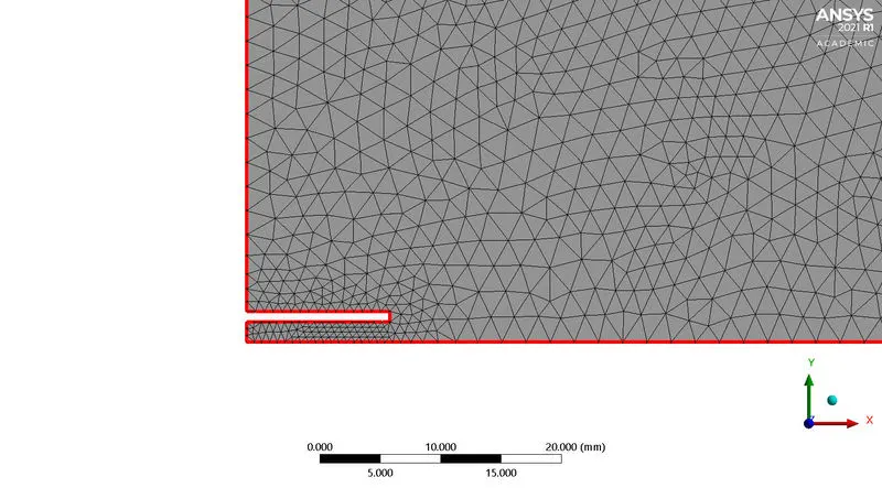
- The surface is meshed with capture proximity of 3 cells and a mesh size of 2mm.
- Air and fuel inlets, outlet and axis are named.
- In fluent, standard k-epsilon model is used.
- Energy equation is enabled.
- For the first part of this study, in species model, methane-air is used as mixture material and for the second part of this study, methane-air-2 step mixuture model is used.
- Next, at air inlet the velocity of air is considered as 5m/s and mass fraction of air is 0.23.
- At fuel inlet, fuel velocity is considered to be 80m/s and fuel mass fraction is given as 1.
- For 2 part of this study, the fuel mole fraction is varied between 0.7 to 1. The mole fraction of water is also varied from 0.05 to 0.3.
- Solution is hybrid initialized.
- Contours for temperature, mass fractions of CO2, N2, H2O, NOX, soot are created.
- Solution is run for 1500 iterations.
- In the post processor, lines are created at 8 different locations in the combustor model to understand the variation of exhaust and soot formation.
- A chart is created to plot the variations.
- Mass averaged values of NOX and soot are parameterized for comparison.
3. Pre-processing:
3.1 Geometry:
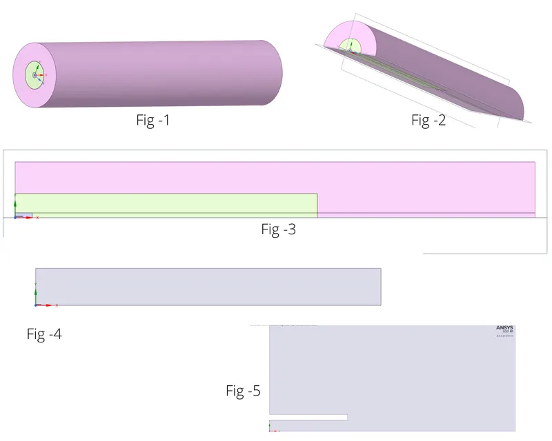
The combustor model is imported to spaceclaim and using split body option, a 2D surface of the model is created for simulation. The below figures represent the creation and merging of 2D surface. The dimensions of the 2D surface is 0.792m*0.08264m. Similar surface with custom dimensions can be created to visualize the results.
3.2 Mesh
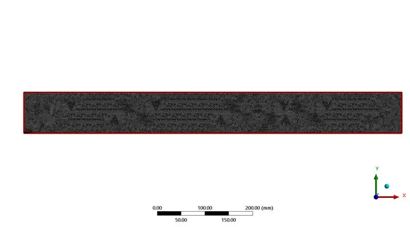
The mesh size used for this study is 2mm. Other mesh details are as mentioned in the table below:
|
Mesh parameter |
Value |
|
No of nodes |
19320 |
|
No of elements |
37706 |
|
Proximity min size |
2e-2mm |
|
Number of cells across gap |
3 |
Below images represent the meshed surface. Triangular elements are used for meshing.
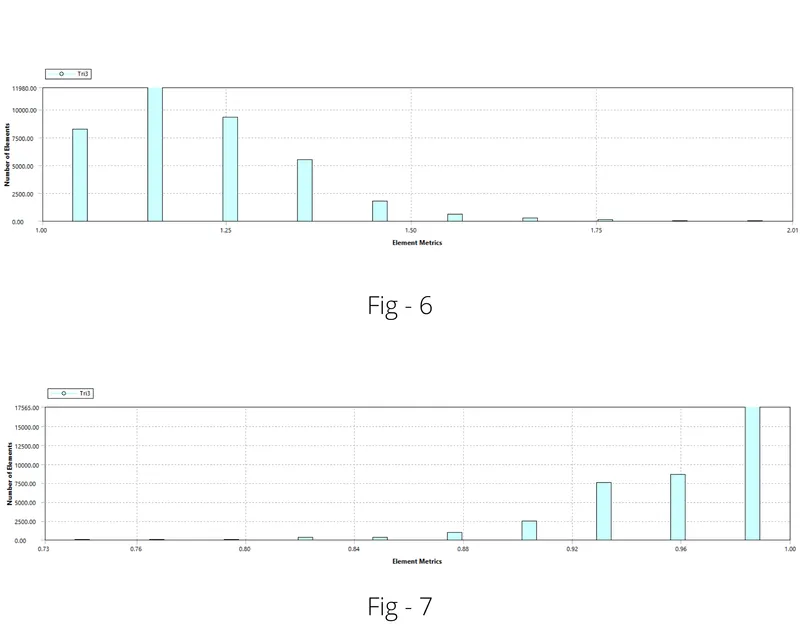
Below image represents the aspect ratio of cells. It can be seen that most of the cells have aspect ratio near 1 in fig-6 and fig-7 indicates the element quality, where only few elements are of bad quality. To visualize the results and understand them, it is found that current mesh size and quality is enough.
3.3 Solver:
For this study, pressure based solver is used. Also the velocity of fuel and oxidant are high enough to be considered turbulent. Standard k-epsilon model with realizable wall function is enabled. The flow field in this study is not too accurate and k-epsilon model has good convergence rate and low memory requirements. Hence, it is selected.
The below image indicates the settings for using species model option for mixture without water. To simulate mixture with water or to add water to fuel, methane-air-2step option needs to be selected. Also as there is no external heat source to initiate combustion, the combustion is governed by turbulence which is enabled through eddy-dissipation interaction. This also provides results quickly.
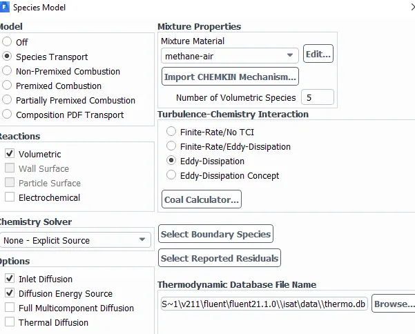
Other boundary conditions considered for this study are as follows:
|
Air inlet velocity |
5m/s |
|
Fuel inlet velocity |
80m/s |
|
Temperature at both inlets |
300k |
|
Mass fraction of Oxygen |
0.23 |
|
Mole fraction of Methane |
1 for part1 |
|
0.7-0.95 for part2 |
|
|
Mass fraction of water |
0.05-0.3 for part2 |
The results of this study can be divided into part 1 and 2. In part 1, the air-methane mixture is simulated for combustion without water and in part 2, the mixture is simulated with water.
4. Results:
4.1 Part-1: Air-methane mixture without water
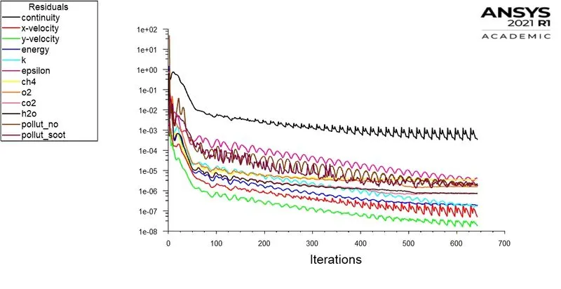
- The solution converged at around 180 iterations. Still the simulation was continued to make sure complete results are obtained.
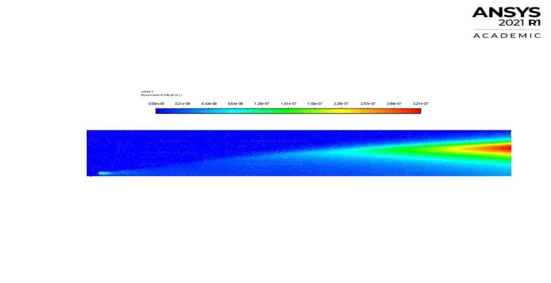
- In the above images, the first one indicates pollutants mass fraction. It can be seen that the pollutants are high at the outlet. They are carried from the inlet as they are formed, which accumulates at the end.
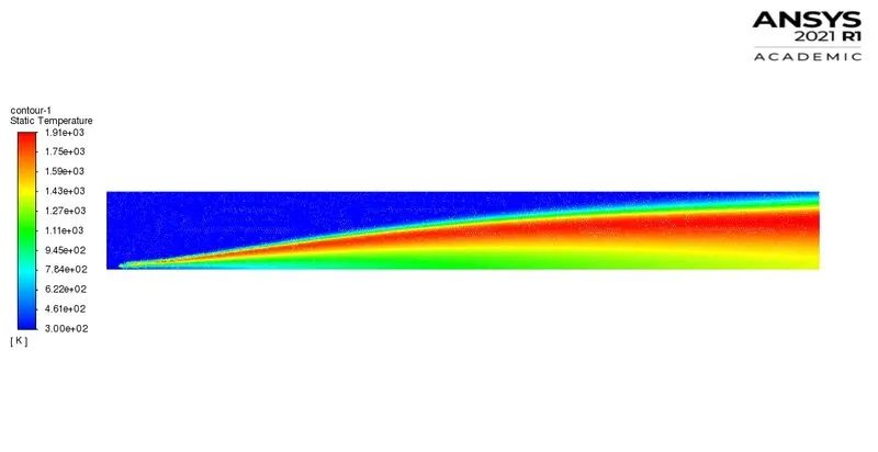
- The second image indicates temperature contour. As the combustion progresses, the temperature increases as well. This is due to the formation of hot exhaust gases which ultimately accumulate at the end and also the increased interaction of fuel and oxidant as their mass fractions increase in the combustor model.
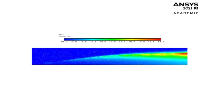
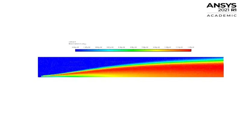
- Soot formation should be avoided as much as possible and the same is addressed in part-2 results of this study. The first of the above images represent soot mass fraction. This can be explained in a similar manner of pollutant formation. As the intensity of combustion increases, formation of soot also proportionately increases. This increase affects the effectiveness of combustion which can be seen at the outlet.
- The second image is the mass fraction of CO2. The fuel inlet is a smaller one at the bottom of the model and it has high velocity. Some of the fuel coming through inlet will not reach the entire width of the model due to its velocity.
- At places where fuel level is higher, CO2 formation is also higher. A small green line can be observed, where it seem like the fuel has lower reach to form high amount of CO2.
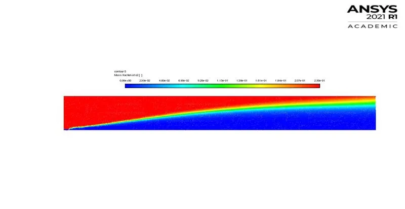
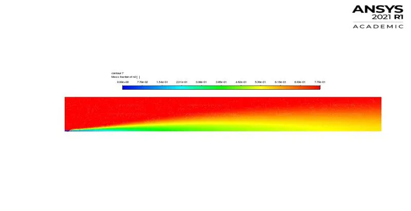
- The first of the above images indicate the mass fraction of oxygen. Oxygen enters through the bigger inlet and hence major portion of oxygen's mass fraction is shown on top of the combustor model.
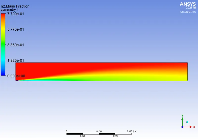
- The second image indicates the mass fraction of nitrogen. As nitrogen only forms oxides, its mass fraction is distributed throughout the model.
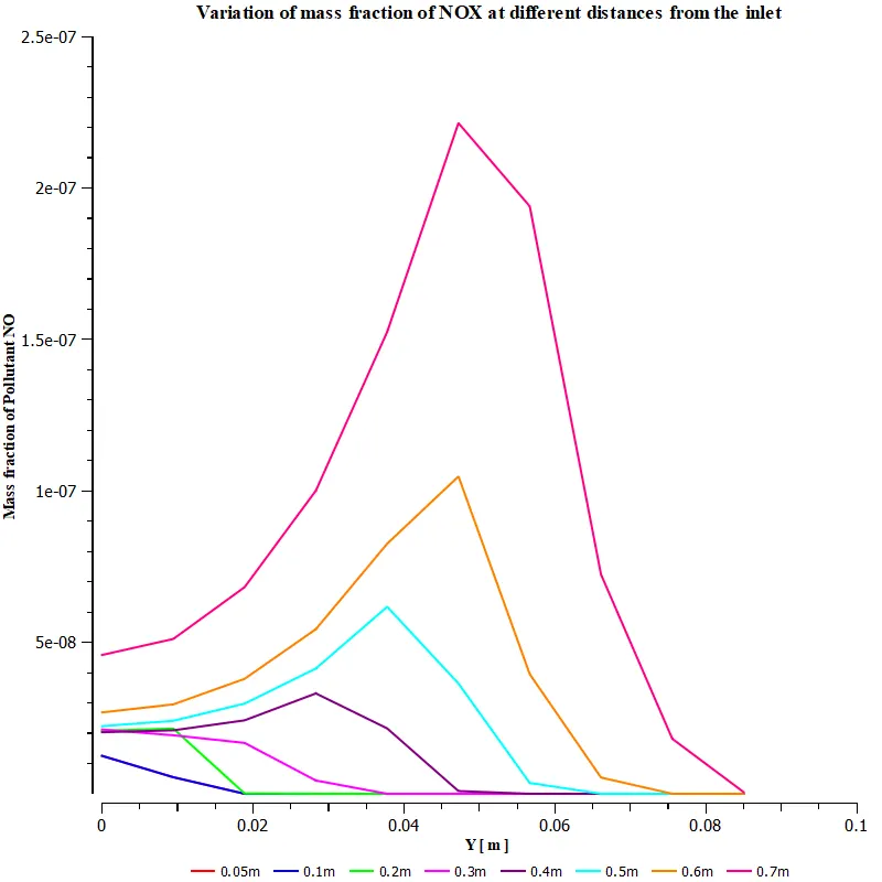
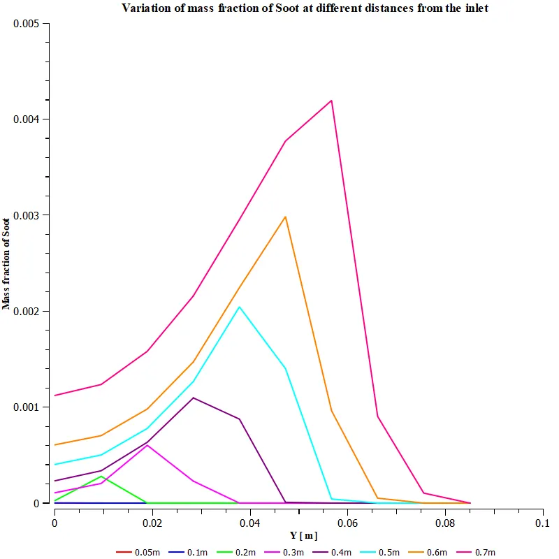
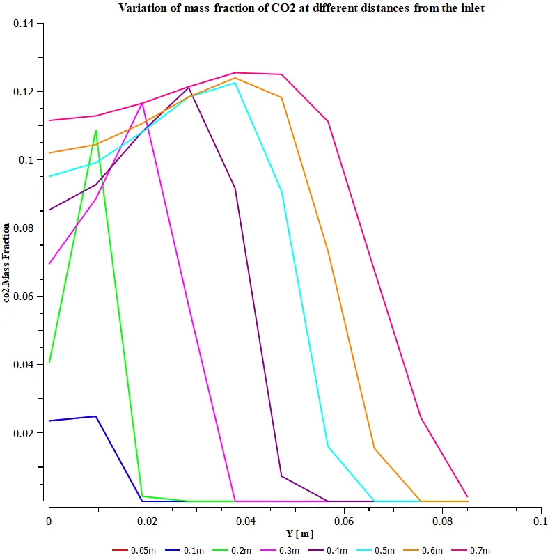
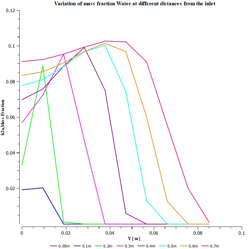
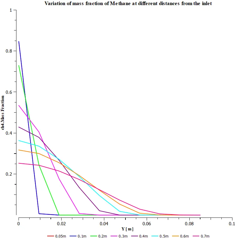
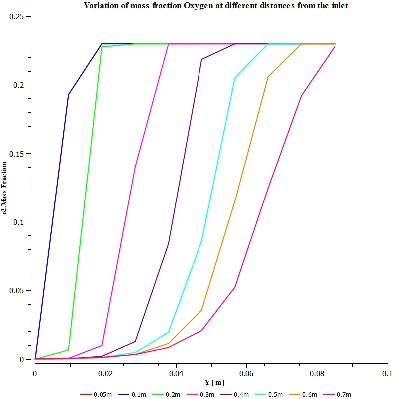
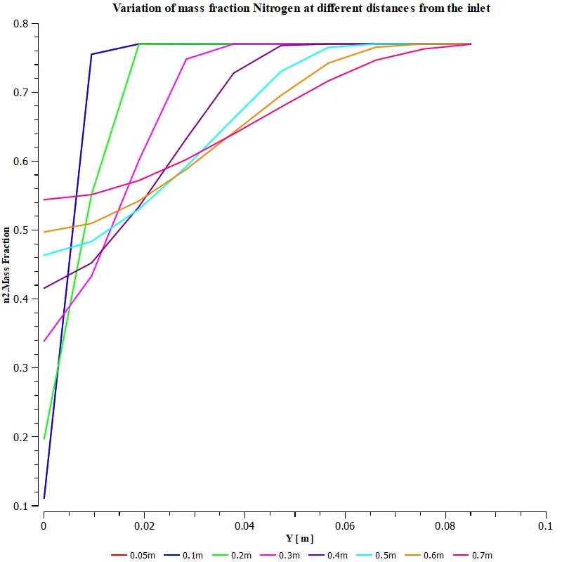
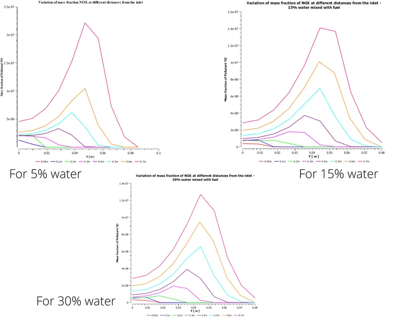
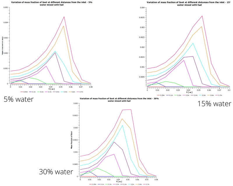
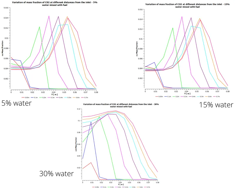
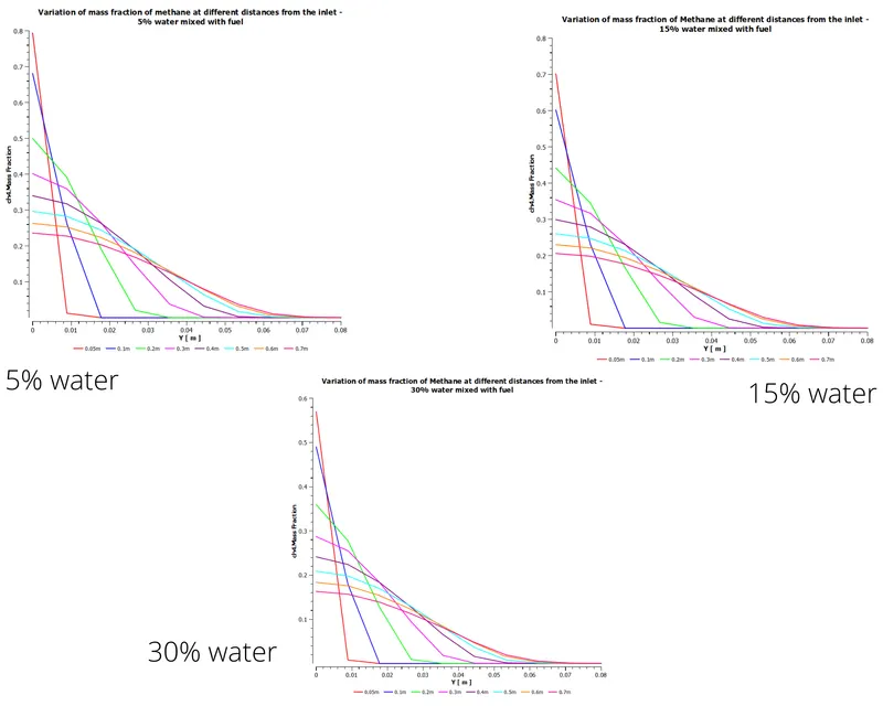
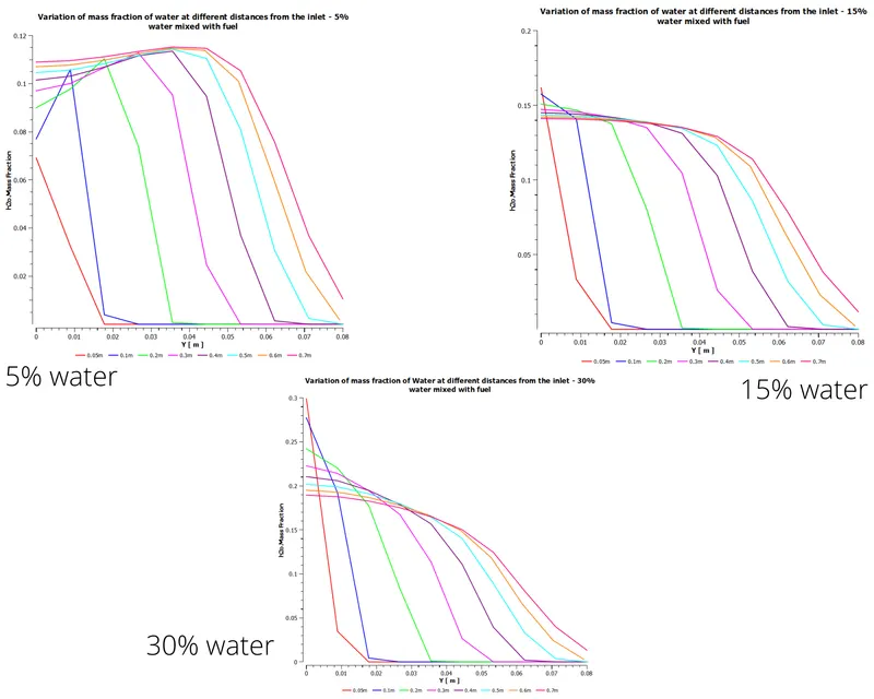
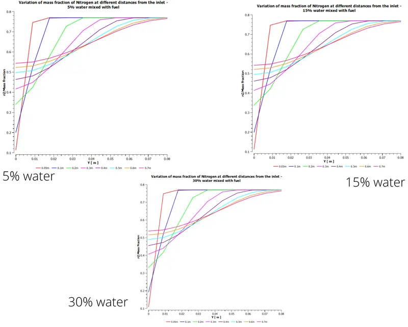
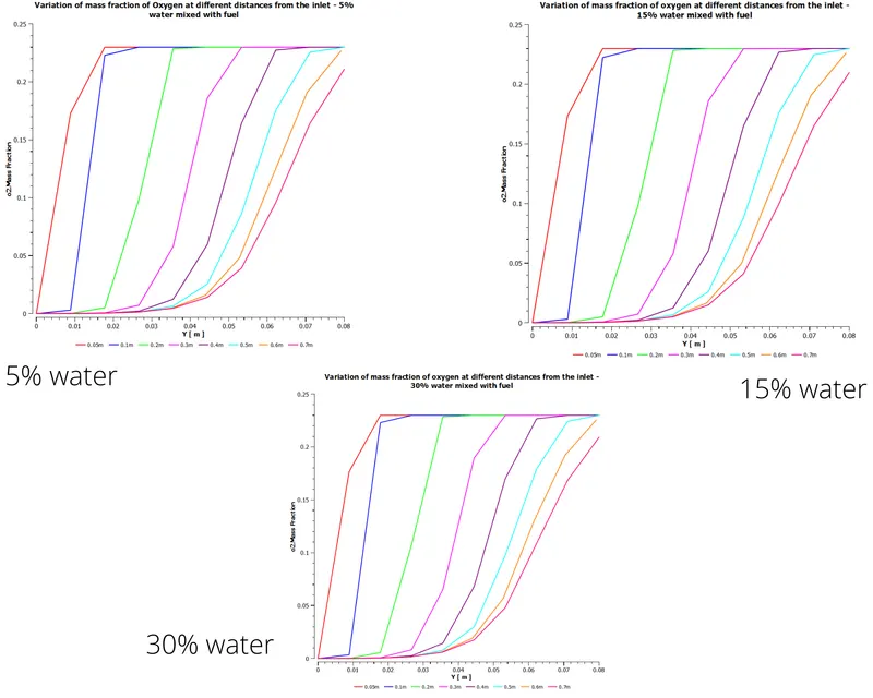
- In all of the above charts variation of mass fraction of different species is shown at different locations from the inlet. The results can be explained similar to the mass fraction contours.
- Only fuel and oxygen consumptions decrease as the process moves towards inlet.
- Due to the velocity values of fuel and oxidant, all of the species reach high mass fraction values at vertical half way of the combustor model. This can also be due to the high intensity of the process happening half way vertical of the combustor.
- As the horizontal distance increases, the interaction of fuel of oxidant also increases and this leads to increase in mass fraction of all the exhausts.
4.2 Part-2: Air-Methane mixture with 5%, 15% and 30% of water
Residuals of simulatio:
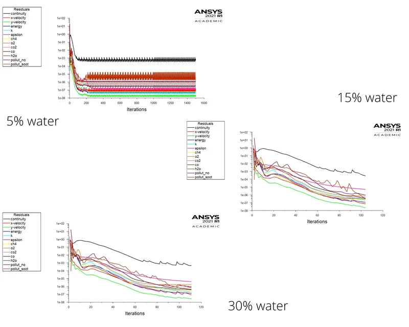
- Simulation with 5% of water did not converge and ran 1500 iterations, where 15% and 30% water simulations converged at 104 and 111 iterations respectively.
4.2.1 Temperature contours:
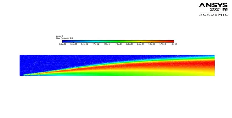
5% water
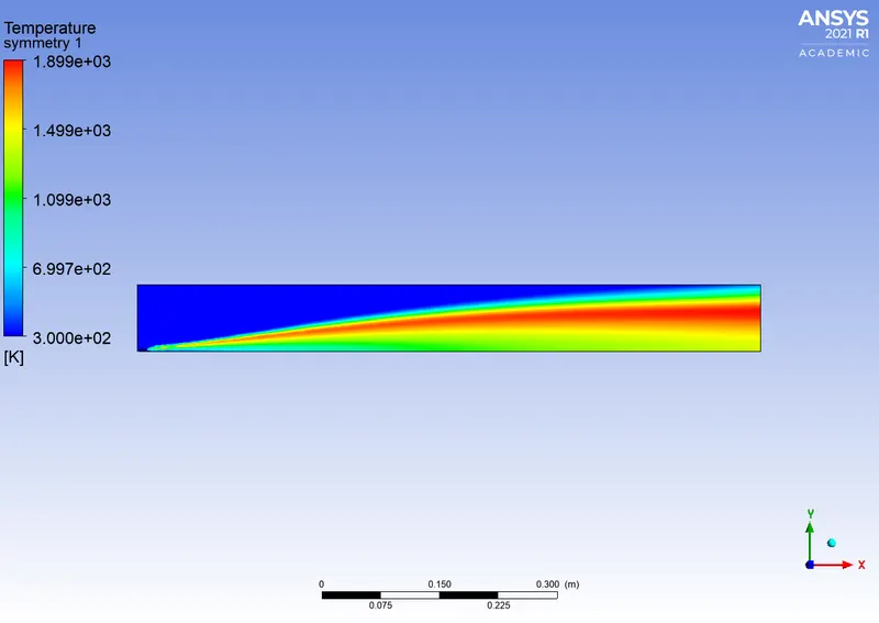
15% water
30% water
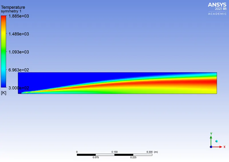
- Temperature distribution remains same irrespective of water addition and it can be seen in the above images.
4.2.2 Pollutants mass fraction contours:
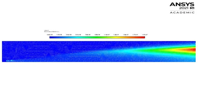
5% water:
15% water:
30% water:
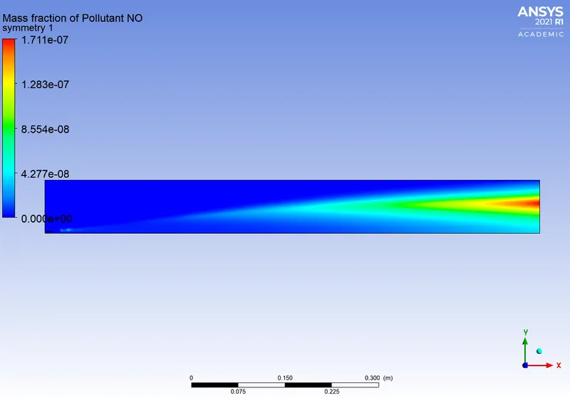
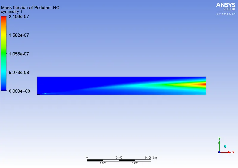
- The difference in mass fraction distribution is very less. It can be observed that as the water % increases, the distribution of pollutants in the green and blue range of the contour increases and the red region decreases in width at a very small rate.
4.2.3 Soot mass fraction contours:
5% water:
15% water:
30%water:
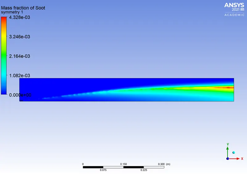
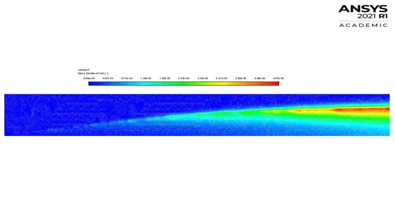
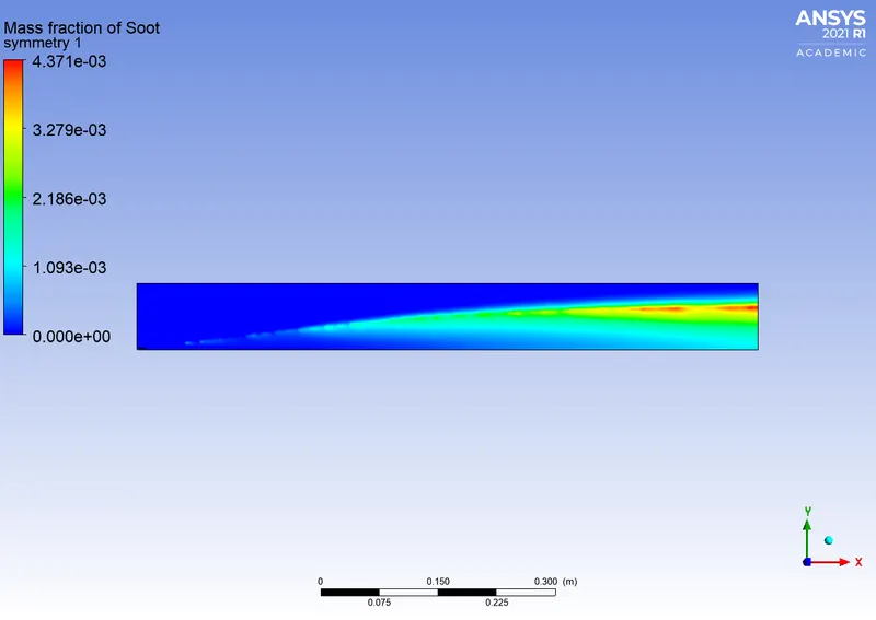
- Mass fraction of soot varies similar to the pollutants. With the addition of water in fuel, soot mass fraction is observed to decrease.
- By comparing the part-1 and part-2 results, it can inferred that the low concentration of soot is more distributed in cases where water is added - this can be observed in the above images.
- And the high concentration of soot, is found to diminish to smaller width.
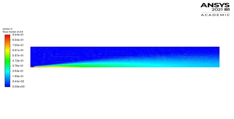
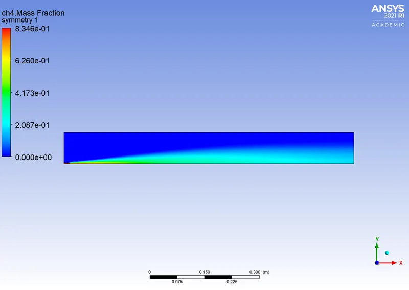
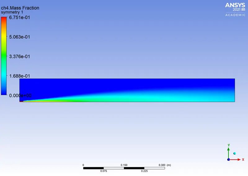
4.2.4 Methane mass fraction contours:
5% water:
15% water:
30% water:
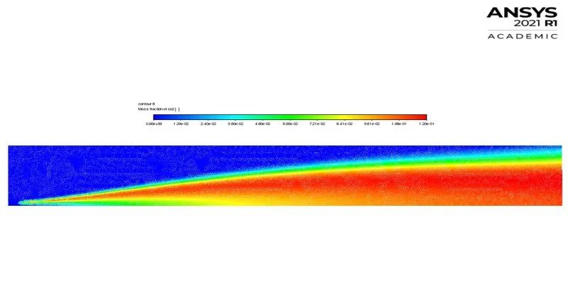
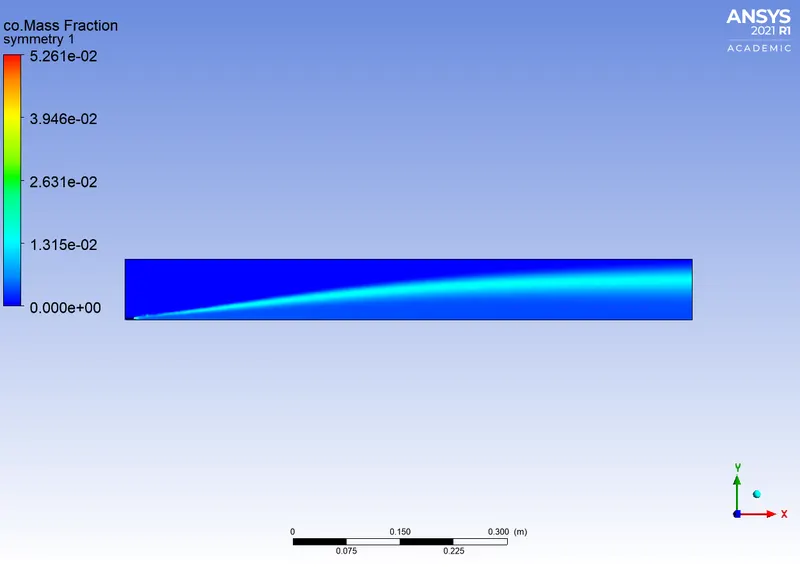
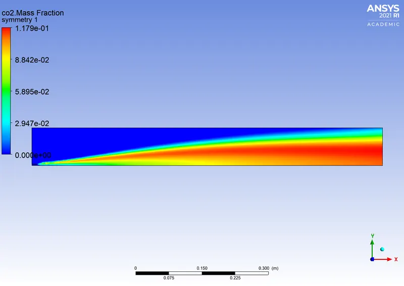
4.2.5 Carbon dioxide and carbon monoxide mass fraction contours:
5% water:
15% water:
30% water:
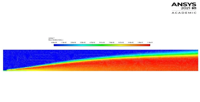
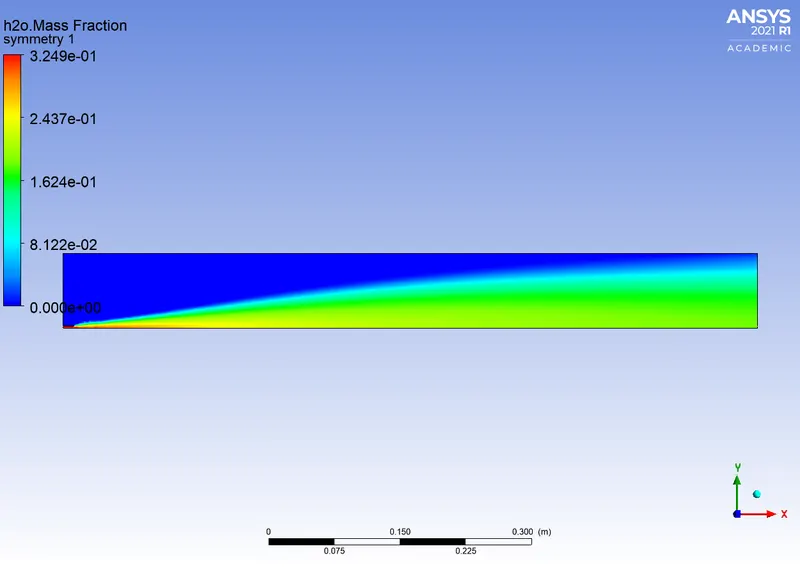
4.2.6 Water mass fraction contours:
5% water:
15% water:
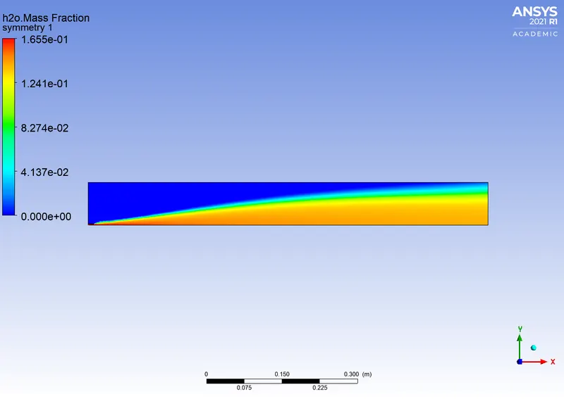
30% water:
4.2.7 Nitrogen mass fraction contours:
5% water
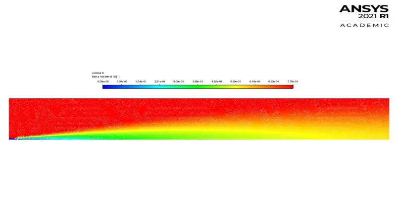
15% water:
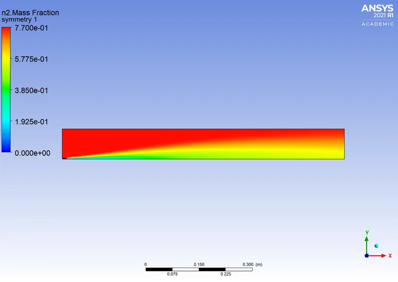
30% water:
4.3 Charts:
4.3.1 Pollutants:
4.3.2 Soot:
4.3.3 Carbon dioxide:
4.3.4 Methane:
4.3.5 Water:
4.3.6 Nitrogen:
4.3.7 Oxygen:
5. Conclusions:
|
Entities to be compared |
Simulation without water |
Simulation with water |
||
|
5% of water |
15% of water |
30% of water |
||
|
NOx mass fraction at the outlet |
1.3202703E-08 |
7.287E-09 |
8.2475073E-09 |
7.6022692E-09 |
|
Soot mass fraction at the outlet |
0.00028367392 |
0.00021365 |
0.00021316977 |
0.0001821077 |
- Pollutants and soot mass fractions decrease with the increase of water concentration in fuel. This can be observed in the above table.
- All of the exhaust species are high in mass fraction at half of vertical distance of combustor model.
- Formation of soot and NOx can be controlled through addition of water, but one also need to keep track of the combustion effectiveness and decide the optimum quantity of water.
6. References: