Adiabatic Flame Temperature calculation

Aim: To calculate Adiabatic Flame Temperature using Python and Cantera for the below mentioned cases

1. AFT variation with Equivalence ratio - in constant volume chamber
2. AFT variation with Heat loss - in constant pressure chamber
3. AFT variation with the type of fuel - Alkane, Alkene and Alkyne
4. AFT variation with the type of fuel - by changing the number of carbon atoms

1. Introduction:

Adiabatic flame temperature is the maximum temperature attained during combustion of particular fuel at constant pressure or constant temperature. AFT depends on lower heating value and high heating value of the fuel.

Lower heating value is the amount of energy that can be extracted from a fuel without considering the latent heat of vapourization of water in the products. This means that water will remain the vapor state and the energy contained within the water vapor will not be released. Hence the combustion products will be at a lower temperature. This causes heat loss. Heat loss effect on AFT is shown in case 2.

2. Coding Approach:

• Necessary libraries such mathplotlib, numpy, cantera, etc are imported.
• A function is created to calculate the enthalpy of individual species on reactants and products side. For this, temperature and thermodynamic co-efficients are considered as inputs.
• Another function to calculate the enthalpy difference between reactants and products is created. Temperature is maintained as a fixed input and based on different cases, other inputs such as phi(equivalence ratio) and fuel are considered.
• One more function to calculate the forward differencing is created. The inputs to this function are similar to the ones mentioned in the above point.
• Guessed temperature value, tolerance and under relaxation factor is defined.
• A for loop and a while loop is created to calculate the AFT values using Newton Rhapson technique.
• AFT is calculated using cantera for case1 and for other cases results are plotted.

3. Cases:

3.1. Case 1: Adiabatic flame temperature variation with Equivalence ratio (In constant volume-chamber)

import matplotlib.pyplot as plt
import math
import numpy as py 
import cantera as ct

def h(T, coeffs):

	R = 8.314 #J/mol-k
	a1 = coeffs[0]
	a2 = coeffs[1]
	a3 = coeffs[2]
	a4 = coeffs[3]
	a5 = coeffs[4]
	a6 = coeffs[5]

	return (a1 + a2*T/2 + a3*pow(T,2)/3 + a4*pow(T,3)/4 + a5*pow(T,4)/5 + a6/T)*R*T

#Low temperature co-efficients - Reactants
ch4_coeffs_l = [5.14987613E+00, -1.36709788E-02, 4.91800599E-05, -4.84743026E-08, 1.66693956E-11, -1.02466476E+04, -4.64130376E+00]

o2_coeffs_l = [3.78245636E+00, -2.99673416E-03, 9.84730201E-06, -9.68129509E-09, 3.24372837E-12, -1.06394356E+03, 3.65767573E+00]

N2_coeffs_l = [0.03298677E+02, 0.14082404E-02, -0.03963222E-04, 0.05641515E-07, -0.02444854E-10, -0.10208999E+04, 0.03950372E+02]

#High temperature co-efficients - Products
co2_coeffs_h = [3.85746029E+00, 4.41437026E-03, -2.21481404E-06, 5.23490188E-10, -4.72084164E-14, -4.87591660E+04, 2.27163806E+00]

h2o_coeffs_h = [3.03399249E+00, 2.17691804E-03, -1.64072518E-07, -9.70419870E-11, 1.68200992E-14, -3.00042971E+04, 4.96677010E+00]

n2_coeffs_h = [0.02926640E+02, 0.14879768E-02, -0.05684760E-05, 0.10097038E-09, -0.06753351E-13, -0.09227977E+04, 0.05980528E+02]

o2_coeffs_h = [3.28253784E+00, 1.48308754E-03, -7.57966669E-07, 2.09470555E-10, -2.16717794E-14, -1.08845772E+03, 5.45323129E+00]

co_coeffs_h = [ 2.71518561E+00, 2.06252743E-03, -9.98825771E-07, 2.30053008E-10, -2.03647716E-14, -1.41518724E+04, 7.81868772E+00]

x = py.linspace(0.1,2)
phi = x

def f(T,phi):

	R  = 8.314 #kj/kmol-k
	h_co2_p = h(T,co2_coeffs_h)
	h_h20_p = h(T,h2o_coeffs_h)
	h_n2_p = h(T,n2_coeffs_h)
	h_o2_p = h(T,o2_coeffs_h)
	h_co_p = h(T,co_coeffs_h)

	Tstd = 298.15 #k
	h_ch4_r = h(Tstd,ch4_coeffs_l)
	h_02_r = h(Tstd,o2_coeffs_l)
	h_n2_r = h(Tstd,N2_coeffs_l)

	H_reactants = h_ch4_r + (2/phi)*h_02_r + (2/phi)*3.76*h_n2_r
	nRT_r = R*Tstd*(1 + (2/phi) + (2/phi)*3.76)

	if phi < 1:

		H_products = h_co2_p + 2*h_h20_p + (7.52/phi)*h_n2_p + ((2/phi)-2)*h_o2_p
		nRT_p = R*T*(1 + 2 + (7.52/phi) + ((2/phi)-2))			

	elif phi > 1:
		H_products = ((4/phi)-3)*h_co2_p + 2*h_h20_p + (7.52/phi)*h_n2_p + (4-(4/phi))*h_co_p
		nRT_p = R*T*(((4/phi)-3) + 2 + (7.52/phi) + (4-(4/phi)))

	return H_products - H_reactants - nRT_p + nRT_r

def fprime(T,phi):
	return (f(T+1e-6,phi) - f(T,phi))/1e-6

T_guess =  1000
tol = 1e-3 
alpha = 0.2
T_aft = []

for m in range(0,len(phi)):

	while(abs(f(T_guess,phi[m])) > tol):
		T_guess = T_guess - alpha*((f(T_guess,phi[m])/fprime(T_guess,phi[m])))
	T_aft.append(T_guess)

#Calculation of Adiabatic flame temperauture using Cantera
gas = ct.Solution('gri30.xml')
T_ct = []

#For loop to calculate number of moles

for k in range(0,len(phi)):

	Total_moles = 1+(2/phi[k])+(7.52/phi[k])
	CH4_moleFrac =  1/Total_moles
	O2_moleFrac = (2/phi[k])/Total_moles
	N2_moleFrac = (7.52/phi[k])/Total_moles

	gas.TPX = 298.15,101325,{'CH4':CH4_moleFrac,'O2':O2_moleFrac,'N2':N2_moleFrac}
	gas.equilibrate('UV','auto')
	T_ct.append(gas.T)

plt.plot(phi,T_aft,color='green',label='Python')
plt.plot(phi,T_ct,color='red',label='Cantera')
plt.legend()
plt.xlabel('Equivalence Ratio')
plt.ylabel('Adiabatic Flame Temperature')
plt.title('Variation of Adiabatic Flame Temperature of Methane wrt Equivalence Ratio')
plt.show()

3.1.1 Results:

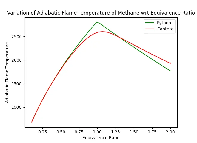
• In the above plot, it can be observed AFT calculated using Cantera is bit less than AFT calculated using Python.
• This is because, in Python, only a few products are considered for the calculation. In reality, there will be a lot of intermediary reactions which leads to more number of products. Cantera considers more number of products for the calculation.
• Hence, due to higher number of products, AFT is less in Cantera.
• Also, for lean mixtures, AFT variation is steep compared to that of rich mixtures. AFT is maximum for a equivalence ratio 1 as shown in the above plot.

3.2. Case 2: Flame temperature variation with Heat loss (In constant pressure-chamber)

import matplotlib.pyplot as plt
import math
import numpy as py 

def h(T, coeffs):

	R = 8.314 #J/mol-k
	a1 = coeffs[0]
	a2 = coeffs[1]
	a3 = coeffs[2]
	a4 = coeffs[3]
	a5 = coeffs[4]
	a6 = coeffs[5]

	return (a1 + a2*T/2 + a3*pow(T,2)/3 + a4*pow(T,3)/4 + a5*pow(T,4)/5 + a6/T)*R*T

#Low temperature co-efficients - Reactants
ch4_coeffs_l = [5.14987613E+00, -1.36709788E-02, 4.91800599E-05, -4.84743026E-08, 1.66693956E-11, -1.02466476E+04, -4.64130376E+00]

o2_coeffs_l = [3.78245636E+00, -2.99673416E-03, 9.84730201E-06, -9.68129509E-09, 3.24372837E-12, -1.06394356E+03, 3.65767573E+00]

N2_coeffs_l = [0.03298677E+02, 0.14082404E-02, -0.03963222E-04, 0.05641515E-07, -0.02444854E-10, -0.10208999E+04, 0.03950372E+02]

#High temperature co-efficients - Products
co2_coeffs_h = [3.85746029E+00, 4.41437026E-03, -2.21481404E-06, 5.23490188E-10, -4.72084164E-14, -4.87591660E+04, 2.27163806E+00]

h2o_coeffs_h = [3.03399249E+00, 2.17691804E-03, -1.64072518E-07, -9.70419870E-11, 1.68200992E-14, -3.00042971E+04, 4.96677010E+00]

n2_coeffs_h = [0.02926640E+02, 0.14879768E-02, -0.05684760E-05, 0.10097038E-09, -0.06753351E-13, -0.09227977E+04, 0.05980528E+02]

o2_coeffs_h = [3.28253784E+00, 1.48308754E-03, -7.57966669E-07, 2.09470555E-10, -2.16717794E-14, -1.08845772E+03, 5.45323129E+00]

co_coeffs_h = [ 2.71518561E+00, 2.06252743E-03, -9.98825771E-07, 2.30053008E-10, -2.03647716E-14, -1.41518724E+04, 7.81868772E+00]

#Low temperature co-efficients - Products for lower heating value
co2_coeffs_l = [2.35677352E+00, 8.98459677E-03, -7.12356269E-06, 2.45919022E-09, -1.43699548E-13, -4.83719697E+04, 9.90105222E+00]

h2o_coeffs_l = [4.19864056E+00, -2.03643410E-03, 6.52040211E-06, -5.48797062E-09, 1.77197817E-12, -3.02937267E+04, -8.49032208E-01]

H_loss_Factor = py.linspace(0,1,10)#input

def f(T,H_loss_Factor):

	R  = 8.314 #kj/kmol-k
	h_co2_p = h(T,co2_coeffs_h)
	h_h2o_p = h(T,h2o_coeffs_h)
	h_n2_p = h(T,n2_coeffs_h)
	h_o2_p = h(T,o2_coeffs_h)
	h_co_p = h(T,co_coeffs_h)

	Tstd = 298.15 #k
	h_ch4_r = h(Tstd,ch4_coeffs_l)
	h_o2_r = h(Tstd,o2_coeffs_l)
	h_n2_r = h(Tstd,N2_coeffs_l)

	h_co2_pl = h(Tstd,co2_coeffs_l)
	h_h2o_pl = h(Tstd,h2o_coeffs_l)
	h_n2_pl = h(Tstd,N2_coeffs_l)

	H_reactants = h_ch4_r + 2*h_o2_r + 2*3.76*h_n2_r

	H_products = h_co2_p + 2*h_h2o_p + 7.52*h_n2_p

	LHV = H_loss_Factor*((h_ch4_r + 2* h_o2_r + 7.52*h_n2_r) - (h_co2_pl + 2*h_h2o_pl + 7.52*h_n2_pl))

	H_loss_max = (H_products - H_reactants + LHV)

	return H_loss_max

def fprime(T,H_loss_Factor):
	return (f(T+1e-6,H_loss_Factor) - f(T,H_loss_Factor))/1e-6

T_guess =  1000
tol = 1e-3 
alpha = 0.2
T_aft = []

for m in range(0,len(H_loss_Factor)):

	while(abs(f(T_guess,H_loss_Factor[m])) > tol):
		T_guess = T_guess - alpha*((f(T_guess,H_loss_Factor[m])/fprime(T_guess,H_loss_Factor[m])))

	T_aft.append(T_guess)

plt.plot(H_loss_Factor,T_aft)
plt.xlabel('H_loss_Factor')
plt.ylabel('Adiabatic Flame Temperature')
plt.title('Variation of AFT wrt Heat Loss')
plt.show()

3.2.1 Results:

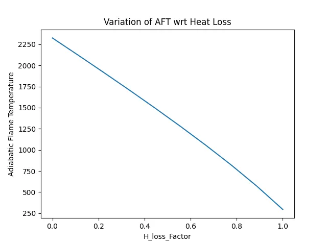
• In the above plot, it can be seen that as the heat loss factor increases the AFT decreases. This is associated with lower heating value of the fuel.
• Heat loss is essentially due to the unobsorbed latent heat of vaporization of water, due to which the other products of combustion stay at lower temperatures, which decreases AFT.

3.3. Case 3: Adiabatic flame temperature variation with respect to Alkane, Alkene, Alkyne

import matplotlib.pyplot as plt
import math
import numpy as py 

def h(T, coeffs):

	R = 8.314 #J/mol-k
	a1 = coeffs[0]
	a2 = coeffs[1]
	a3 = coeffs[2]
	a4 = coeffs[3]
	a5 = coeffs[4]
	a6 = coeffs[5]

	return (a1 + a2*T/2 + a3*pow(T,2)/3 + a4*pow(T,3)/4 + a5*pow(T,4)/5 + a6/T)*R*T

#Low temperature co-efficients - Reactants
c2h6_coeffs_l = [4.29142492E+00, -5.50154270E-03, 5.99438288E-05, -7.08466285E-08, 2.68685771E-11, -1.15222055E+04, 2.66682316E+00]#Ethane

c2h4_coeffs_l = [3.95920148E+00, -7.57052247E-03, 5.70990292E-05, -6.91588753E-08, 2.69884373E-11, 5.08977593E+03, 4.09733096E+00]#Ethene

c2h2_coeffs_l = [8.08681094E-01, 2.33615629E-02, -3.55171815E-05, 2.80152437E-08, -8.50072974E-12, 2.64289807E+04, 1.39397051E+01]#Acetylene

o2_coeffs_l = [3.78245636E+00, -2.99673416E-03, 9.84730201E-06, -9.68129509E-09, 3.24372837E-12, -1.06394356E+03, 3.65767573E+00]

N2_coeffs_l = [0.03298677E+02, 0.14082404E-02, -0.03963222E-04, 0.05641515E-07, -0.02444854E-10, -0.10208999E+04, 0.03950372E+02]

#High temperature co-efficients - Products
co2_coeffs_h = [3.85746029E+00, 4.41437026E-03, -2.21481404E-06, 5.23490188E-10, -4.72084164E-14, -4.87591660E+04, 2.27163806E+00]

h2o_coeffs_h = [3.03399249E+00, 2.17691804E-03, -1.64072518E-07, -9.70419870E-11, 1.68200992E-14, -3.00042971E+04, 4.96677010E+00]

n2_coeffs_h = [0.02926640E+02, 0.14879768E-02, -0.05684760E-05, 0.10097038E-09, -0.06753351E-13, -0.09227977E+04, 0.05980528E+02]

Tstd = 298.15 #k
Ethane  = h(Tstd,c2h6_coeffs_l)
Ethene  = h(Tstd,c2h4_coeffs_l)
Acetylene = h(Tstd,c2h2_coeffs_l)

Fuel = [Ethane,Ethene,Acetylene]

def f(T,Fuel):

	R  = 8.314 #kj/kmol-k
	h_co2_p = h(T,co2_coeffs_h)
	h_h2o_p = h(T,h2o_coeffs_h)
	h_n2_p = h(T,n2_coeffs_h)

	h_o2_r = h(Tstd,o2_coeffs_l) 
	h_n2_r = h(Tstd,N2_coeffs_l)

	if Fuel == Ethane:
		H_reactants = Ethane + 3.5*h_o2_r + 3.5*3.76*h_n2_r
		H_products = 2*h_co2_p + 3*h_h2o_p + 3.5*3.76*h_n2_p

	elif Fuel == Ethene:
		H_reactants = Ethene + 3*h_o2_r + 3*3.76*h_n2_r
		H_products = 2*h_co2_p + 2*h_h2o_p + 3*3.76*h_n2_p

	else:
		H_reactants = Acetylene + 2.5*h_o2_r + 2.5*3.76*h_n2_r
		H_products = 2*h_co2_p + 2*h_h2o_p + 2.5*3.76*h_n2_p

	return (H_products - H_reactants)

def fprime(T,Fuel):
	return (f(T+1e-6,Fuel) - f(T,Fuel))/1e-6

T_guess =  1000
tol = 1e-3 
alpha = 0.2
T_aft = []

for t in Fuel:

	while(abs(f(T_guess,t)) > tol):
		T_guess = T_guess - alpha*((f(T_guess,t)/fprime(T_guess,t)))

	T_aft.append(T_guess)
plt.plot(['Ethane','Ethene','Acetylene'],T_aft)
plt.xlabel('Fuel')
plt.ylabel('Adiabatic Flame Temperature')
plt.title('Variation of AFT wrt Alkane, Alkene and Alkyne')
plt.bar(['Ethane','Ethene','Acetylene'],T_aft)
plt.show()

3.3.1 Results:

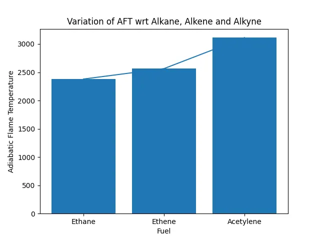
• The bond energy between carbon atoms is higher. Triple bond between just the two carbon atoms contains 812 kj/mol of bond energy. Hence more energy must be supplied to break triple bonds.
• This high energy is the reason for higher AFTs in alkynes as shown in the above plot.

3.4. Case 4: Adiabatic flame temperature variation with respect to number of Carbon atom chains

import matplotlib.pyplot as plt
import math
import numpy as py 

def h(T, coeffs):

	R = 8.314 #J/mol-k
	a1 = coeffs[0]
	a2 = coeffs[1]
	a3 = coeffs[2]
	a4 = coeffs[3]
	a5 = coeffs[4]
	a6 = coeffs[5]

	return (a1 + a2*T/2 + a3*pow(T,2)/3 + a4*pow(T,3)/4 + a5*pow(T,4)/5 + a6/T)*R*T

#Low temperature co-efficients - Reactants
ch4_coeffs_l = [5.14987613E+00, -1.36709788E-02, 4.91800599E-05, -4.84743026E-08, 1.66693956E-11, -1.02466476E+04, -4.64130376E+00]#Methane

c2h6_coeffs_l = [4.29142492E+00, -5.50154270E-03, 5.99438288E-05, -7.08466285E-08, 2.68685771E-11, -1.15222055E+04, 2.66682316E+00]#Ethane

c3h8_coeffs_l = [0.93355381E+00, 0.26424579E-01, 0.61059727E-05, -0.21977499E-07, 0.95149253E-11, -0.13958520E+05, 0.19201691E+02]#Propane

o2_coeffs_l = [3.78245636E+00, -2.99673416E-03, 9.84730201E-06, -9.68129509E-09, 3.24372837E-12, -1.06394356E+03, 3.65767573E+00]

N2_coeffs_l = [0.03298677E+02, 0.14082404E-02, -0.03963222E-04, 0.05641515E-07, -0.02444854E-10, -0.10208999E+04, 0.03950372E+02]

#High temperature co-efficients - Products
co2_coeffs_h = [3.85746029E+00, 4.41437026E-03, -2.21481404E-06, 5.23490188E-10, -4.72084164E-14, -4.87591660E+04, 2.27163806E+00]

h2o_coeffs_h = [3.03399249E+00, 2.17691804E-03, -1.64072518E-07, -9.70419870E-11, 1.68200992E-14, -3.00042971E+04, 4.96677010E+00]

n2_coeffs_h = [0.02926640E+02, 0.14879768E-02, -0.05684760E-05, 0.10097038E-09, -0.06753351E-13, -0.09227977E+04, 0.05980528E+02]

Tstd = 298.15 #k
Methane  = h(Tstd,ch4_coeffs_l)
Ethane  = h(Tstd,c2h6_coeffs_l)
Propane  = h(Tstd,c3h8_coeffs_l)

Fuel = [Methane,Ethane,Propane]

def f(T,Fuel):

	R  = 8.314 #kj/kmol-k
	h_co2_p = h(T,co2_coeffs_h)
	h_h2o_p = h(T,h2o_coeffs_h)
	h_n2_p = h(T,n2_coeffs_h)

	h_o2_r = h(Tstd,o2_coeffs_l) 
	h_n2_r = h(Tstd,N2_coeffs_l)

	if Fuel == Ethane:
		H_reactants = Ethane + 3.5*h_o2_r + 3.5*3.76*h_n2_r
		H_products = 2*h_co2_p + 3*h_h2o_p + 3.5*3.76*h_n2_p

	elif Fuel == Methane:
		H_reactants = Methane + 2*h_o2_r + 2*3.76*h_n2_r
		H_products = h_co2_p + 2*h_h2o_p + 2*3.76*h_n2_p

	else:
		H_reactants = Propane + 5*h_o2_r + 5*3.76*h_n2_r
		H_products = 3*h_co2_p + 4*h_h2o_p + 5*3.76*h_n2_p

	return (H_products - H_reactants)

def fprime(T,Fuel):
	return (f(T+1e-6,Fuel) - f(T,Fuel))/1e-6

T_guess =  1000
tol = 1e-3 
alpha = 0.2
T_aft = []

for t in Fuel:

	while(abs(f(T_guess,t)) > tol):
		T_guess = T_guess - alpha*((f(T_guess,t)/fprime(T_guess,t)))

	T_aft.append(T_guess)
plt.plot(['Methane','Ethane','Propane'],T_aft)
plt.xlabel('Fuel')
plt.ylabel('Adiabatic Flame Temperature')
plt.title('Variation of AFT wrt change in number of Carbon atoms')
plt.bar(['Methane','Ethane','Propane'],T_aft)
plt.show()

3.4.1 Results:

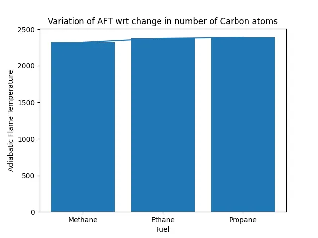
• Higher the number of carbon atoms, stronger the bonds between atoms and hence there is a slight increase in AFT as the number of carbon atoms are increased. This trend is shown in the above plot.

4. References:

1.https://courses.lumenlearning.com/cheminter/chapter/bond-energy/#:~:text=Bond%20Energy%20(kJ%2Fmol)&text=As%20can%20be%20seen%20by,triple%20bonds%20are%20even%20stronger.