Flow over a backward facing step using CONVERGE CFD
Aim: To simulate flow over a backward facing step for mesh sizes -
- dx = dy = dz =2e-3 m
- dx = dy = dz =1.5e-3 m
- dx = dy = dz =1.0e-3 m
1. Introduction:
Study of flow over Backward Facing Step(BFS) is important to understand the features of a separated flow. Separation of flow occurs in so many applications such as airfoils at high angle of attacks, moving automobile, flow around a boat, etc. BFS is a simple geometry used to understand free shear flow separation, vortex evolution and re-attachement.
The flow separation features are characterised by the step length, Reynolds number, pressure force, etc. The below image indicates the four different regions in BFS flow field:
In this study, the flow is driven by pressure difference. So, the pressure at the inlet is higher than pressure at the outlet. As the flow moves near the step, it experiences a sudden decrease in pressure due to which flow separation occurs. This flow separation leads to the formation of primary voritces (larger ones - near the free shear layer) and secondary vortices (smaller ones - near the step corner).
Vortices are formed primarily due to pressure difference. The velocity of fluid particles in the free shear layer is higher and the movement of these particles creates a vacuum type region in the step area. Due to this, the fluid particles are pulled back towards the main flow, thus forming vortices. These vortices and free shear layer combine with the main flow in the reattachment region. At this stage, the flow has reached steady-state.
There are other parameters that affect the separation of flow and formation of vortices such as turbulence. At high Reynolds numbers, flow separation results in vortices with higher energy dissipation rates. This affects the performance of the entire system.
As discussed above, the flow field in BFS in divided into four regions:
- Separated Shear layer.
- Recirculation region under the shear layer.
- Re-attachment region.
- Recovery region.
1.1 Governing equations
The flow is considered to be 2D, Compressible and the equation form is Conservation form. Becuase the the geometry or control volume is fixed in space with fluid moving inside it.
The equations are given by:
- Continuity - `(delrho)/(delt) +nabla.(rhov) = 0`
- Momentum -
- X - component - `(del(rhou))/(delt) + nabla.(rhouV) = -(delP)/(delx) + (del tau_(x.x))/(delx) + (del tau_(y.x))/(dely) + (del tau_(z.x))/(delz) + rho. f_x`
- Y - component - `(del(rhov))/(delt) + nabla.(rhovV) = -(delP)/(dely) + (del tau_(y.y))/(dely) + (del tau_(x.y))/(delx) + (del tau_(z.y))/(delz) + rho. f_y`
- Energy - `del/(delt).[rho (e + v^2/2)] + nabla. [rho (e + v^2/2)*V] = rho.q + del/(delx) (K . (delT)/(delx)) + del/(dely) (K . (delT)/(dely)) - (del(uP))/(delx) - (del(vP))/(dely) + (del(vtau_(xy)))/(delx) + (del(utau_(yx)))/(dely) + (del(vtau_(yy)))/(dely) + (del(utau_(x.x)))/(delx) + rhof. V`
Where 'V' in energy equation is the velocity vector. V = ui+vj
2. Solution Approach:
- Import the geometry to Converge studio and check for defects.
- Define Inlet, outlet, front and back boundaries.
- Chose Time-based application.
- Consider gas-type simulation with air as predefined mixture in materials.
- Select Steady-state solver for the simulation - set number of cycles - 15000.
- Define a volumetric region containing air.
- Define boundary conditions (pressure at inlet and outlet).
- Select RNG K-`epsilon` turbulence model.
- Define grid sizes - 2e-3m, 1.5e-3m, 1e-3m - 3 different cases.
- Export input files to a folder and run the simulation on Cygwin command prompt.
- Convert the post.h files to paraview format and post process the results.
3. Pre-processing:
3.1 Geometry
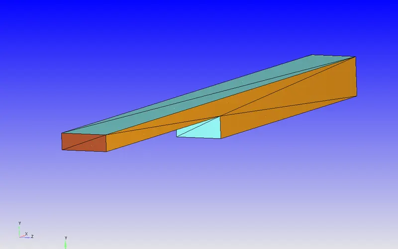
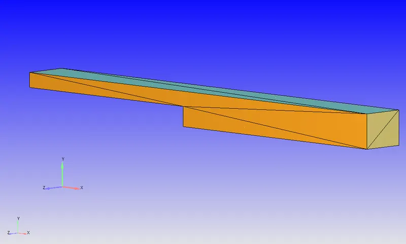
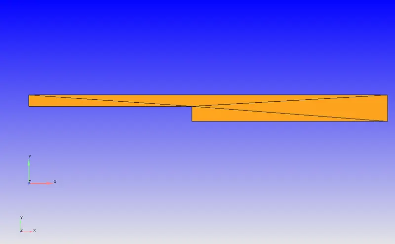
- The geometry is imported (stl format). Dimensions of the geometry is given by - 0.272m*0.01m*0.025m.
3.2 Mesh
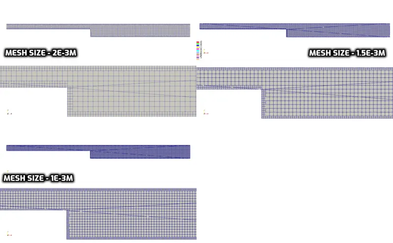
- The above image indicates meshed views for 3 different mesh sizes.
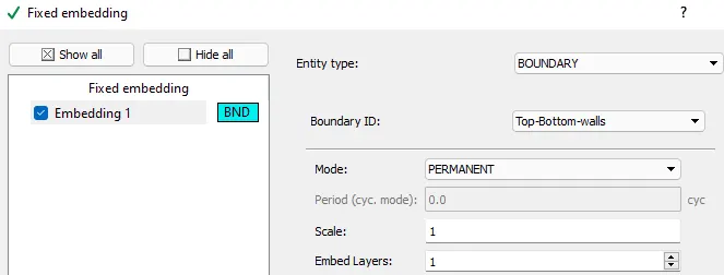
- Embedding is process of refining areas of importance. For this study, the walls of BFS are embedded. The details are shown below:
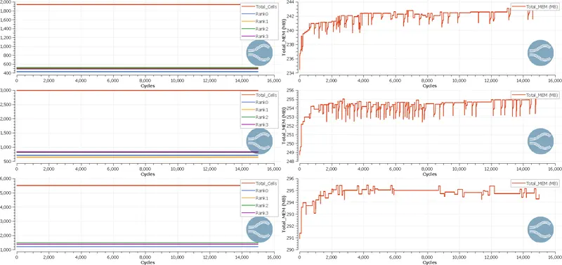
- In the above image, left images indicate the cells count for mesh size 2e-3m, 1.5e-3m and 1e-3m from top to bottom respectively. The right images represent the memory consumption for simulation with different mesh sizes.
- It is clear that the both the number of cells and memory increase with decreasing the mesh size.
- For this study, 4 processors were used in parallel and hence the cell count is shown for 4 processors.
4. Solver:
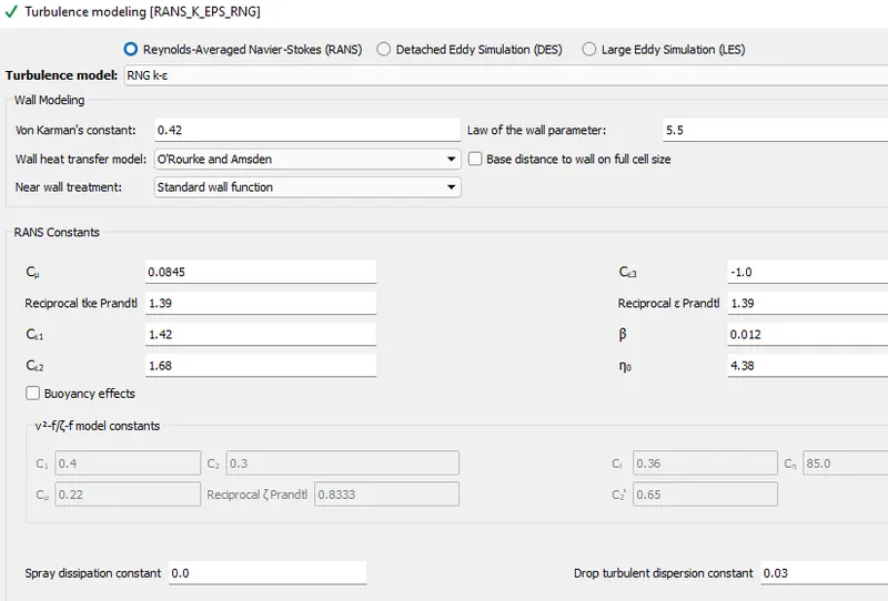
The turbulence model used for this study is RNG K-epsilon model. This model has good convergence rate and low memory requirements compared to other models. Also, this uses wall functions, which means that flow field in the buffer layer is neglected.
The table below contains solver set-up details:
|
Solver set-up details |
||||||
|
Boundary conditions |
Simulation time parameters |
Steady – state monitor details |
||||
|
Regions |
Conditions |
Value |
No of cycles |
15000 |
Min number of cycles to be executed |
15000 |
|
Inlet |
Temperature, Pressure |
300k, 110325pa |
Min time step |
1e-6s |
Monitor start delay |
200 cycles |
|
Outlet |
Temperature, Pressure |
300k, 101325pa |
Max time step |
1s |
Sample size |
100 cycles |
|
Front and back |
2D |
- |
Max convection CFL limit |
0.5 |
Relative tolerance |
0.01 |
|
Top and Bottom |
Wall |
- |
- |
- |
Max std deviation |
0.01 |
5. Post-processing:
In this section, the results pertaining to all the cases are presented.
5.1 Mesh size - 2e-3m
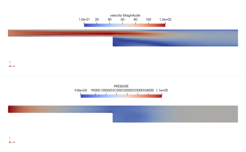
- The above image indicates velocity(top) and pressure contours(bottom).
- The separation zone and reattachment zones can be seen in the velocity contour, but not clearly due to coarser mesh size.
- It can also be seen that the velocity near the step is lesser compared to other areas and due to this lower velocity a region is created near the step called re-circulation region.
- Ahead of this region, the flow re-attaches itself to the main flow and that region is called re-attachment region. Both of these regions are not clearly visible in for mesh size.
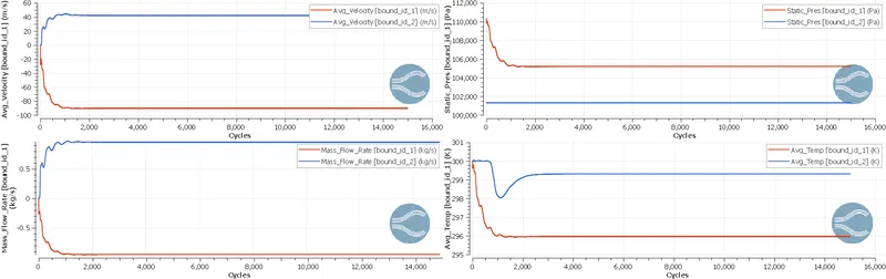
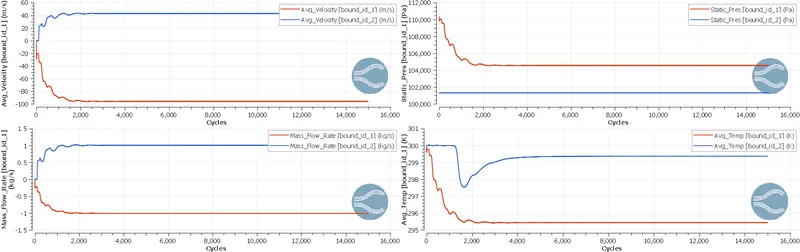
- The principle of conservation of mass can be verified by observing top and bottom images on the left side.
- Increase in velocity and mass flow rate at outlet is proportional to decrease in the variables at inlet.
- The right images indicate avg pressure and temperature at inlet and outlet.
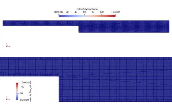
Below is the simulation (gif) of velocity contour:
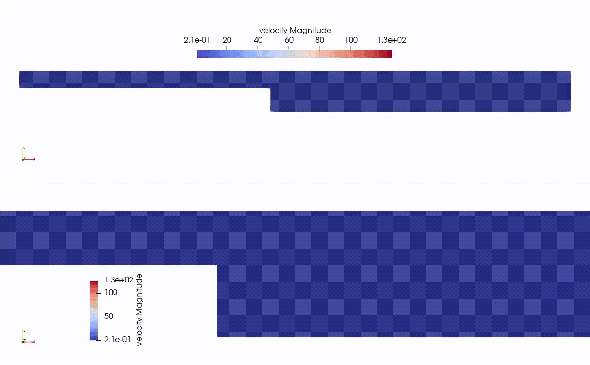
- The results explained in this section hold true for the remaining cases. The only differences are clear visulization and accuracy due to smaller mesh size.
5.2 Mesh size - 1.5e-3m
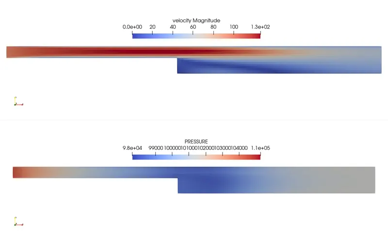
Velocity and pressure contour:
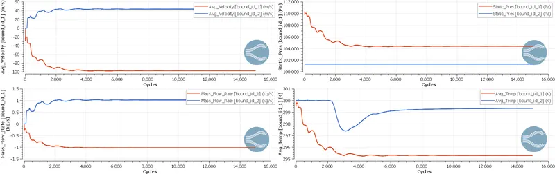
Variation in velocity, mass flow rate, temperature, pressure at inlet and outlet:
Below is the simulation (gif) of velocity contour:
5.3 Mesh size - 1e-3m
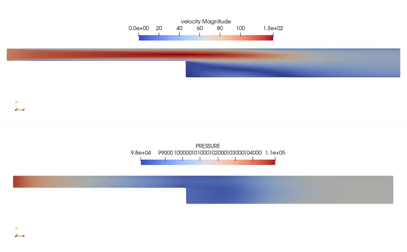
Velocity and pressure contour:
Variation in velocity, mass flow rate, temperature, pressure at inlet and outlet:
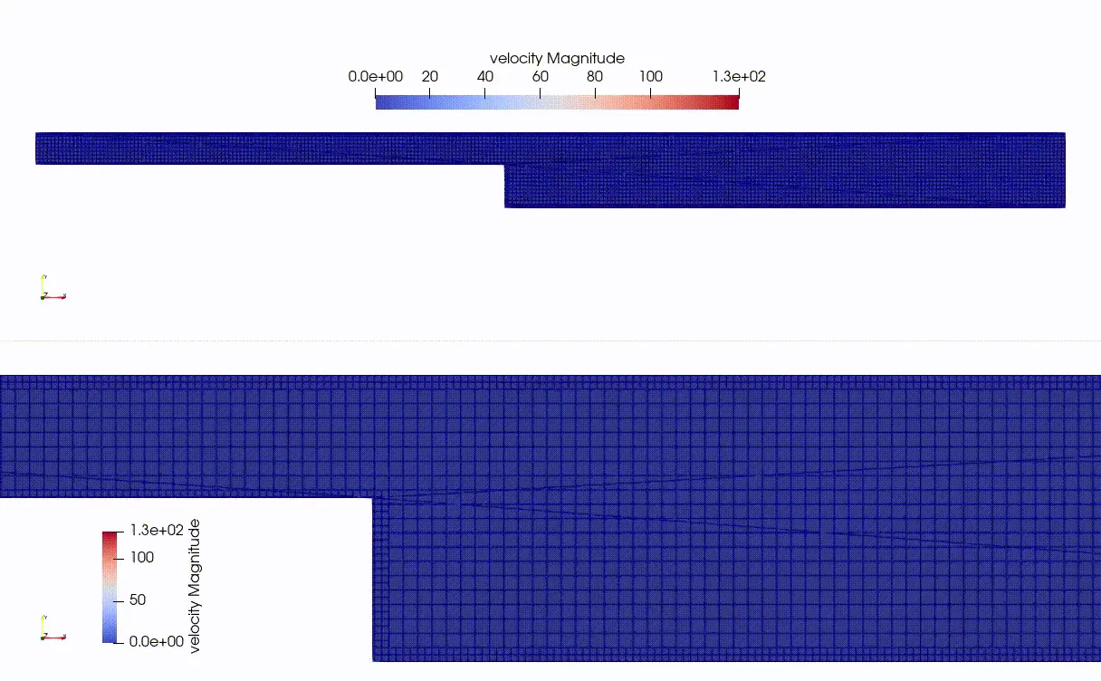
Below is the simulation (gif) of velocity contour:
5.4 Special case
- For this case, the pressure difference is set to be 39,000pa between inlet and outlet and mesh size is set as 2e-4, with the same embedding details as mentioned in the mesh section.
- This is done to observe re-circulation and re-attachment regions clearly.
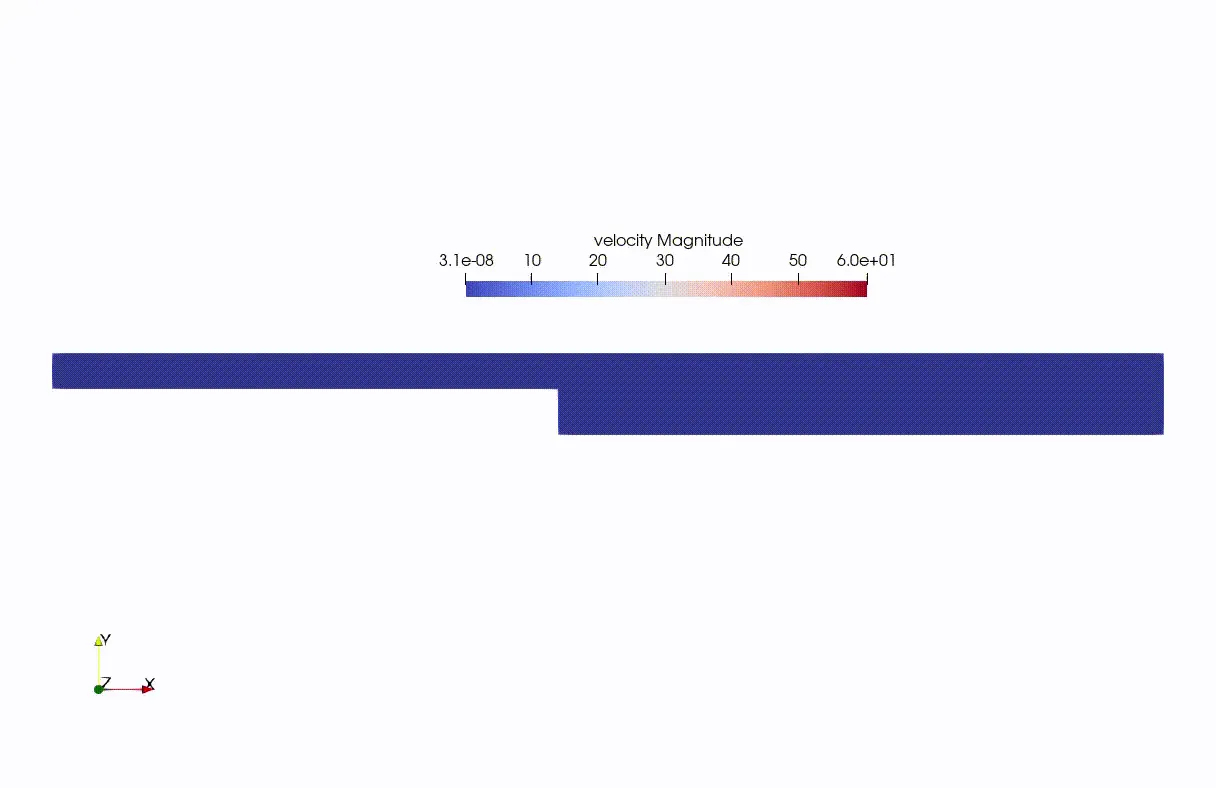
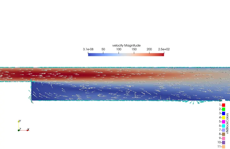
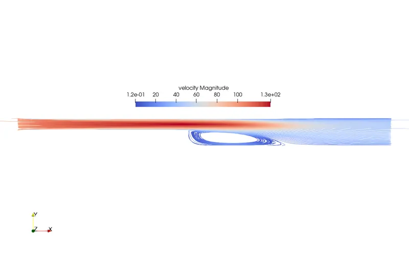
- In the above, the left image shows the re-circulation region in terms of velocity vectors - only pressure difference is changed for this case (case 5.3) and the pressure difference is 39,000pa.
- The right image shows the streamlines of velocity for case 5.3 with no changes.
6. Resources: