week-11 Joint creation and Demonstration
Aim: The joints of revolute, cylindrical, translational and spherical joints between two rigid bodies and two deformable bodies are compared in the Ls-dyna software.
Objective: The joints is part of the machine used to connect two or more parts together temporary or permanently. They will be designed in such a manner, there will be relative motion to these parts by Constraining the degree of freedom or let the constrain free depending on the mechanism.
Procedure:
The revolute joint which is having the hinge joint will be used to in rotation motion. This type of motion is used in the door hinges and uniaxial rotation motion.
The meshed plates are imported with two parts.
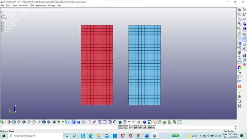
Figure 1: Two meshed parts
The two bodies are considered to be rigid bodies with material properties card as MAT 20_Rigid.
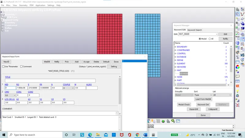
Figure 2: Mat 20_Rigid
The two parts assigned with the section and material ID.
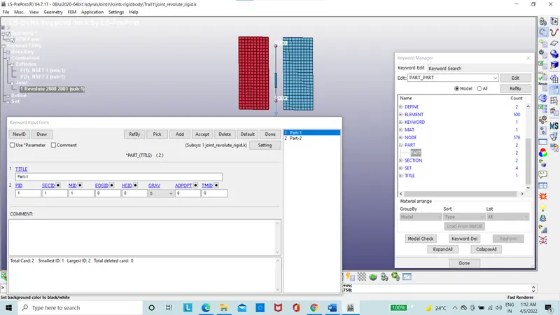
Figure 3: Part Card
The boundary condition for Fixed condition using the SPC is set on for nodes.
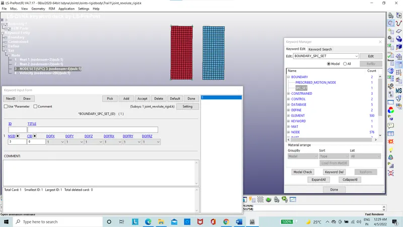
Figure 4: Boundary Spc set with Fixed condition
The Load curve is created using the define option.
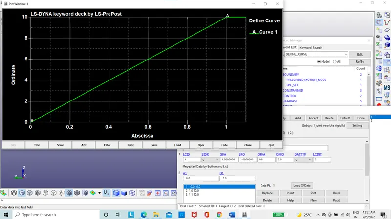
Figure 5: Load curve
The time step is created using the define option.
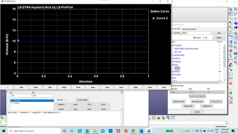
Figure 6: Time step curve
The boundary motion set is created with the displacement with LCID.
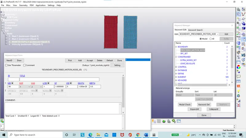
Figure 7: Boundary motion set
The four nodes are created with node ID as 2000, 2001, 2002 and 2003.
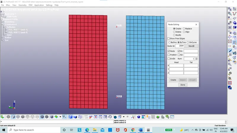
Figure 8: Nodes Coincident with each other
The constrained extra node set is created.
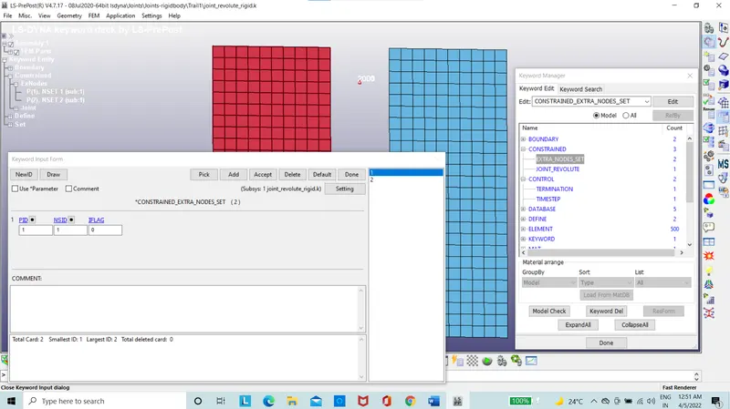
Figure 9: Constrained extra node for Part-1
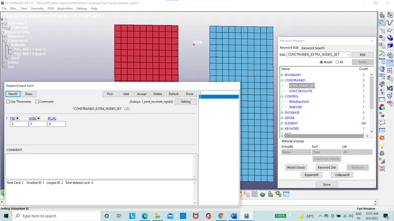
Figure 10: Constrained extra node for Part-2
The revolute joint is made using the constraint option.
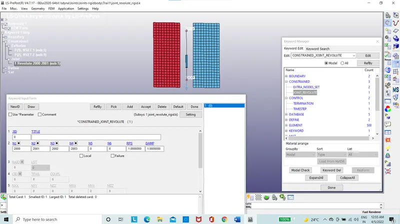
Figure 11: Constrained Revolute Joint
The time step card is used with LCTM input with time step curve.
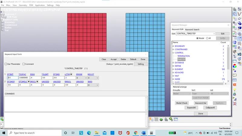
Figure 12: Time step card
The termination card is used.
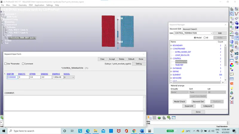
Figure 13: Termination card
The ASCII option is set using the database.
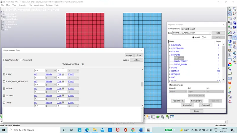
Figure 14: ASCII option.
The binary D3 plot is set using database.
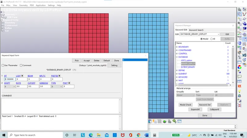
Figure 15: Binary D3plot
The Extent binary is set using the database.
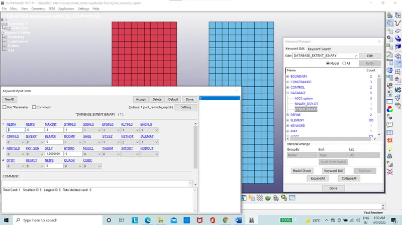
Figure 16: Extent Binary
The keyword File is saved and run.
Here, the two deformable bodies are considered by changing the material and replacing the constrain extra node with the Constrain Nodal rigid body (CNRB) and remaining cards would remain the same for the deformable revolute joint simulation.
The two bodies are considered to be rigid bodies with material properties card as MAT 24_piecewise Linear plasticity.
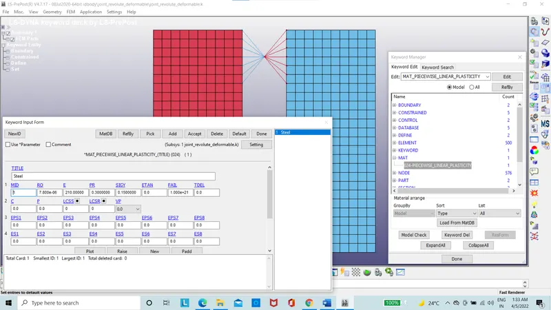
Figure 17: Mat 24_piecewise Linear plasticity
The Constrain Nodal rigid body (CNRB) is created by deleting the constrained extra node card.
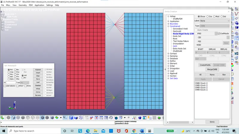
Figure 18: Constrain Nodal rigid body (CNRB)
The file is saved and run.
The Cylindrical joint is having the translational motion of one of the cylindrical joints. This type of motion is used in the journal bearing.
The meshed cylindrical parts are imported with two parts.
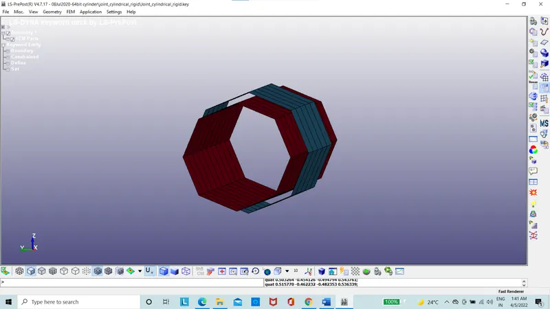
Figure 19: Two meshed parts
The two bodies are considered to be rigid bodies with material properties card as MAT 20_Rigid.
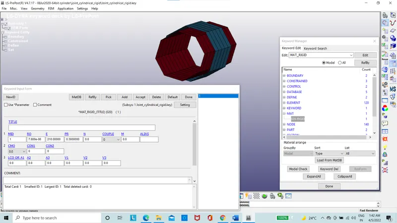
Figure 20: Mat 20_Rigid
The two parts assigned with the section and material ID.
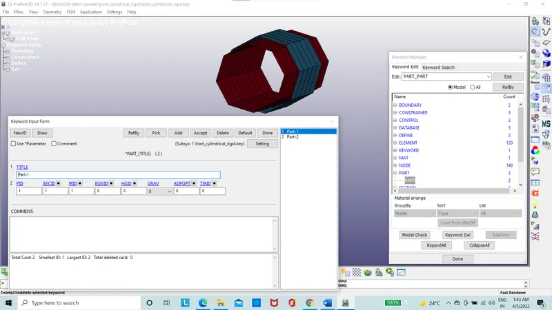
Figure 21: Part Card
The boundary condition for Fixed condition using the SPC is set on for nodes.
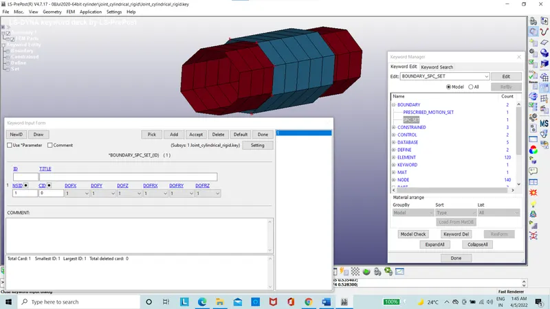
Figure 22: Boundary Spc set with Fixed condition
The Load curve is created using the define option.
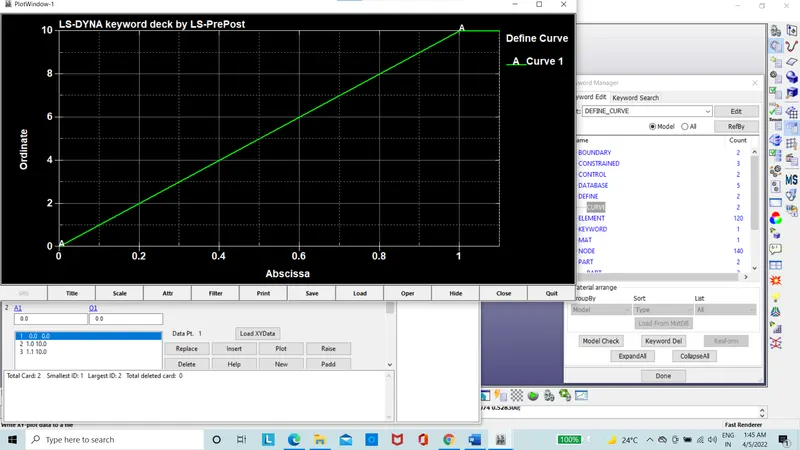
Figure 23: Load curve
The time step is created using the define option.
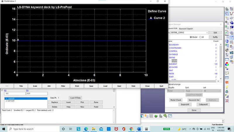
Figure 24: Time step curve
The boundary motion set is created with the displacement with LCID.
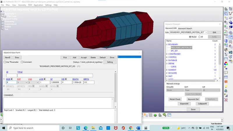
Figure 25: Boundary motion set
The four nodes are created with node ID as 1000, 1001, 1002 and 1003.
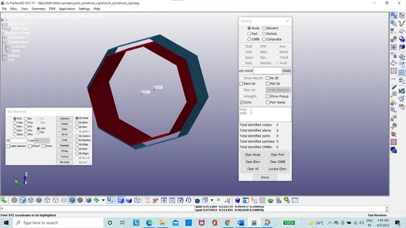
Figure 26: Nodes Coincident with each other
The constrained extra node set is created.
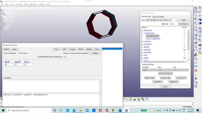
Figure 27: Constrained extra node for Part-1
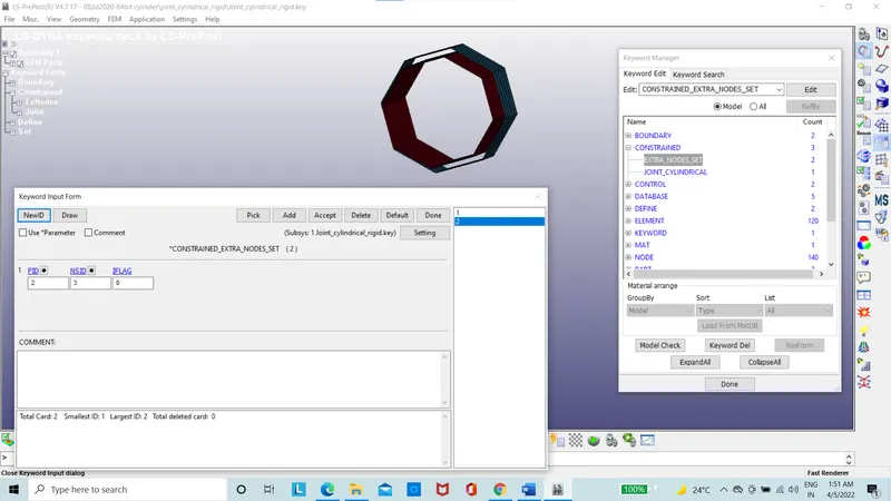
Figure 28: Constrained extra node for Part-2
The revolute joint is made using the constraint option.
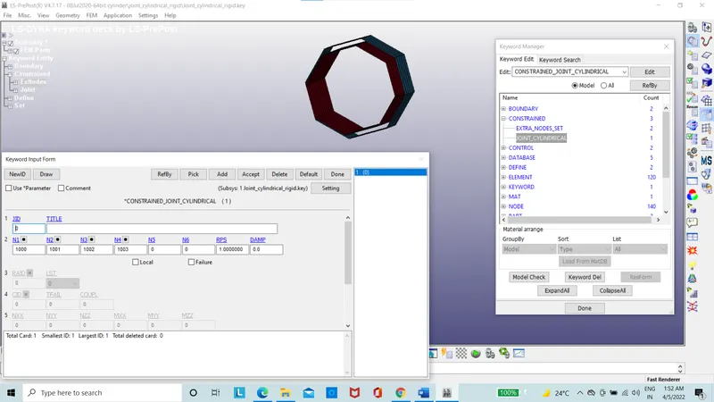
Figure 29: Constrained Cylindrical Joint
The time step card is used with LCTM input with time step curve.
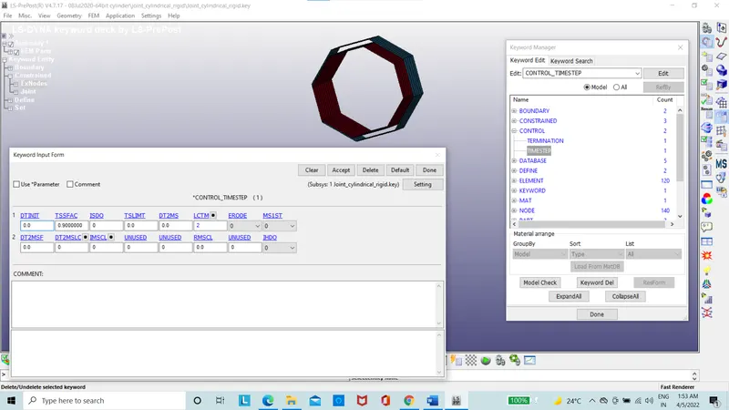
Figure 30: Time step card
The termination card is used.
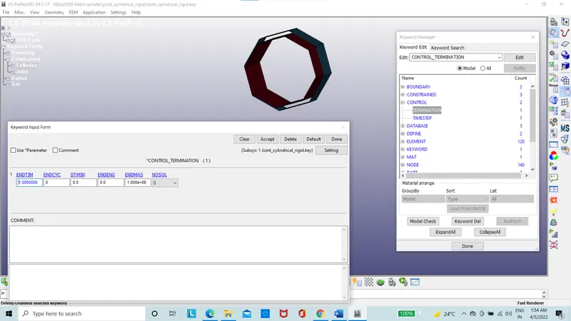
Figure 31: Termination card
The ASCII option is set using the database.
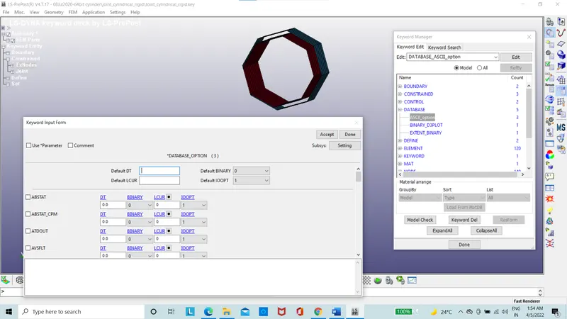
Figure 32: ASCII option.
The binary D3 plot is set using database.
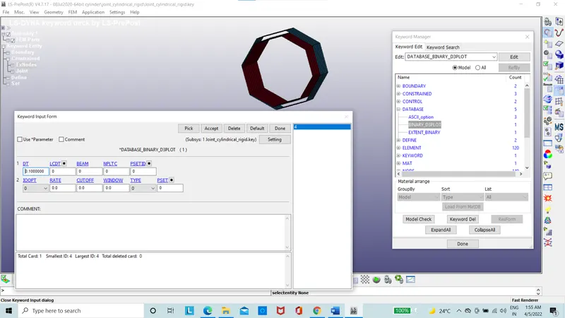
Figure 33: Binary D3plot
The Extent binary is set using the database.
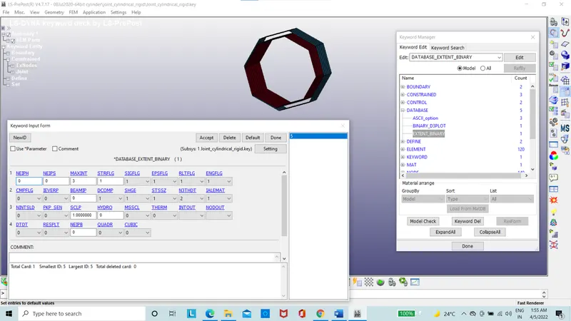
Figure 34: Extent Binary
The keyword File is saved and run.
Here, the two deformable bodies are considered by changing the material and replacing the constrain extra node with the Constrain Nodal rigid body (CNRB) and remaining cards would remain the same for the deformable cylindrical joint simulation.
The two bodies are considered to be rigid bodies with material properties card as MAT 24_piecewise Linear plasticity.
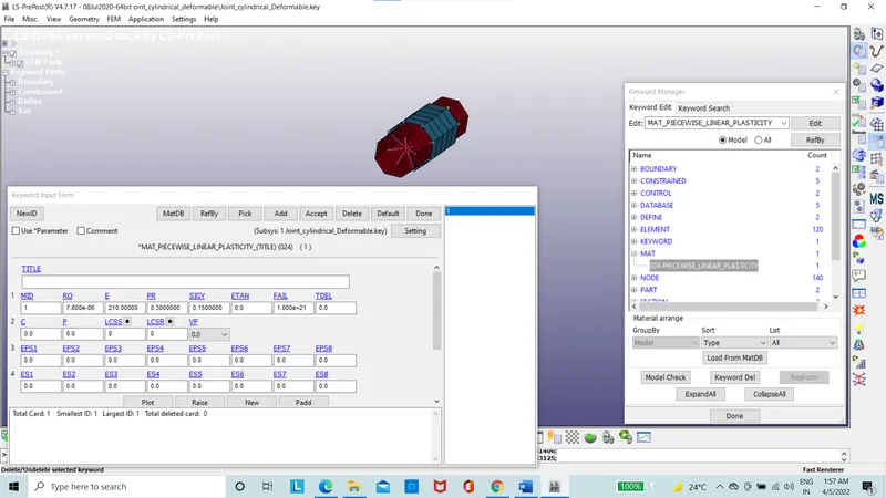
Figure 35: Mat 24_piecewise Linear plasticity
The Constrain Nodal rigid body (CNRB) is created by deleting the constrained extra node card.
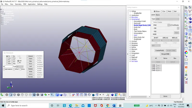
Figure 36: Constrain Nodal rigid body (CNRB)
The file is saved and run.
The translational joint is used for translational motion where it is not free to rotate.
The meshed tubes are imported with two parts.
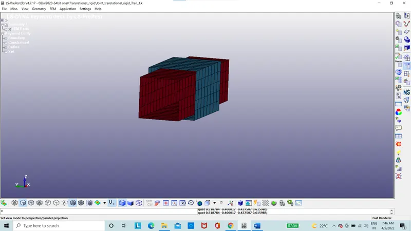
Figure 37: Two meshed parts
The two bodies are considered to be rigid bodies with material properties card as MAT 20_Rigid.
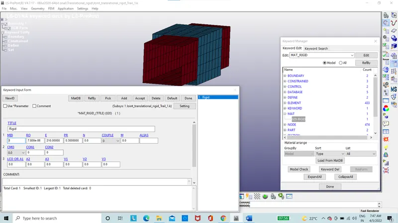
Figure 38: Mat 20_Rigid
The two parts assigned with the section and material ID.
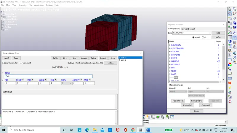
Figure 39: Part Card
The boundary condition for Fixed condition using the SPC is set on for nodes.
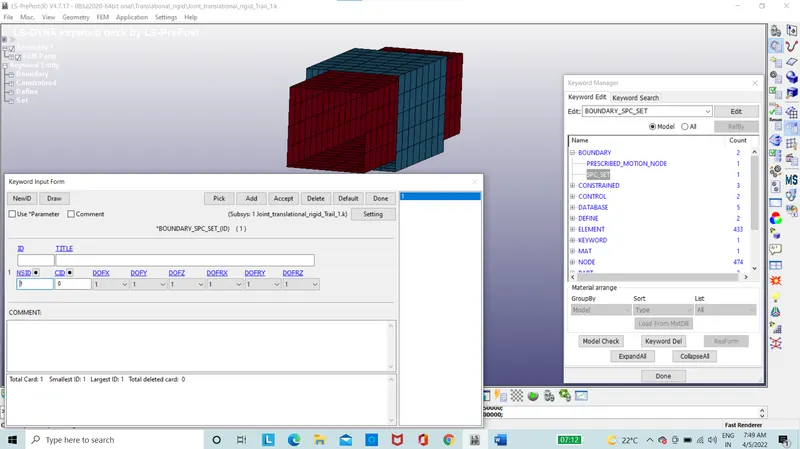
Figure 40: Boundary Spc set with Fixed condition
The Load curve is created using the define option.
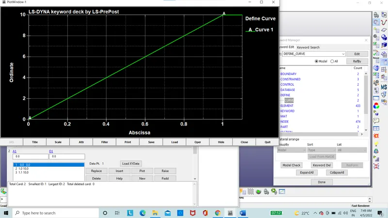
Figure 41: Load curve
The time step is created using the define option.
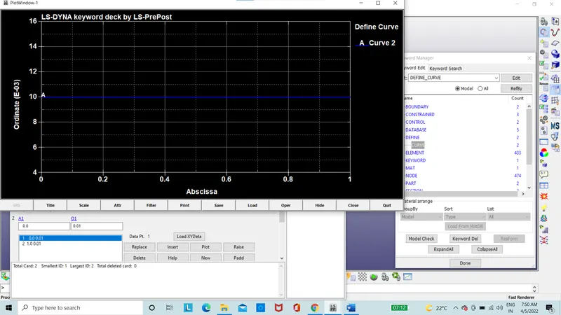
Figure 42: Time step curve
The boundary motion set is created with the displacement with LCID.
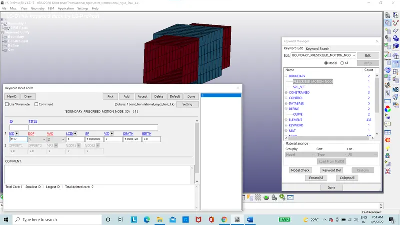
Figure 43: Boundary motion set
The six nodes are created with node ID as 5000, 5001, 5002, 5003, 5004 and 5005.
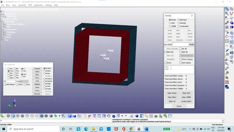
Figure 44: Nodes Coincident with each other
The constrained extra node set is created.
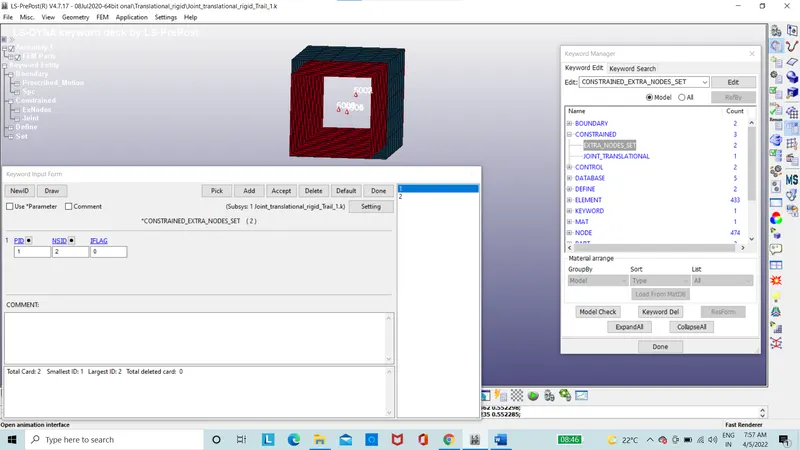
Figure 45: Constrained extra node for Part-1
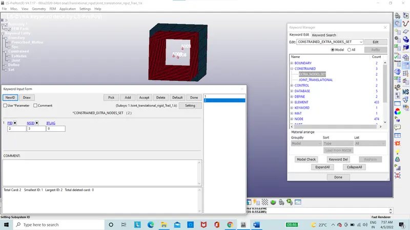
Figure 46: Constrained extra node for Part-2
The revolute joint is made using the constraint option.
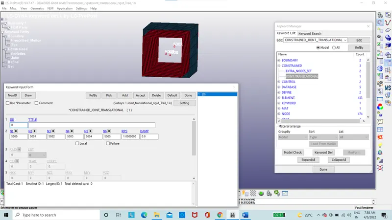
Figure 47: Constrained Translational Joint
The time step card is used with LCTM input with time step curve.
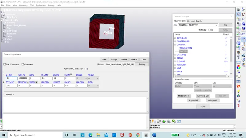
Figure 48: Time step card
The termination card is used.
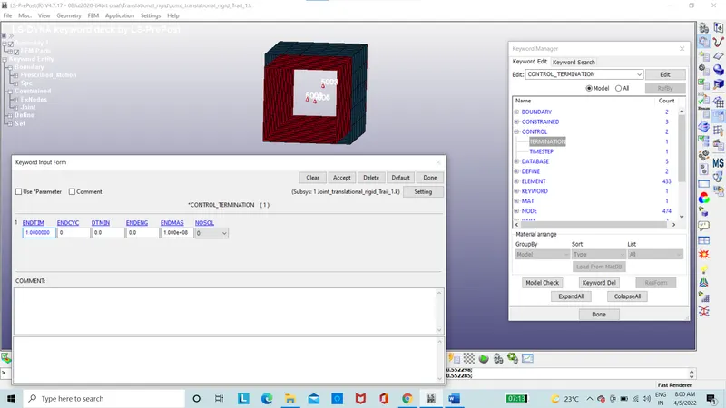
Figure 49: Termination card
The ASCII option is set using the database.
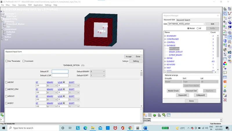
Figure 50: ASCII option.
The binary D3 plot is set using database.
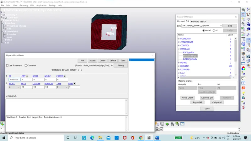
Figure 51: Binary D3plot
The Extent binary is set using the database.
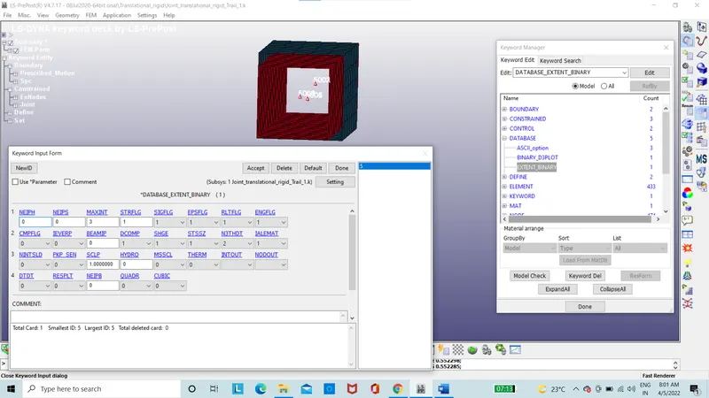
Figure 52: Extent Binary
The keyword File is saved and run.
Here, the two deformable bodies are considered by changing the material and replacing the constrain extra node with the Constrain Nodal rigid body (CNRB) and remaining cards would remain the same for the deformable translational joint simulation.
The two bodies are considered to be rigid bodies with material properties card as MAT 24_piecewise Linear plasticity.
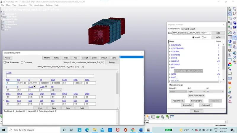
Figure 53: Mat 24_piecewise Linear plasticity
The Constrain Nodal rigid body (CNRB) is created by deleting the constrained extra node card.
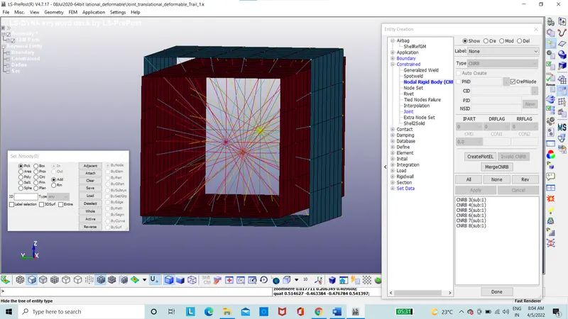
Figure 54: Constrain Nodal rigid body (CNRB)
The file is saved and run.
The spherical joint which will revolve inside in only rotation motion inside in spherical motion. This type of motion is used in rear mirror of a car.
The meshed plates are imported with two parts.
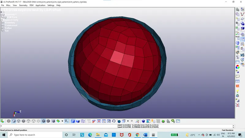
Figure 55: Two meshed parts
The two bodies are considered to be rigid bodies with material properties card as MAT 20_Rigid.
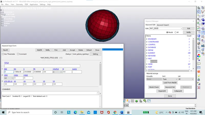
Figure 56: Mat 20_Rigid
The two parts assigned with the section and material ID.
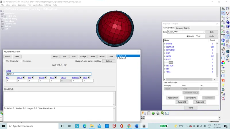
Figure 57: Part Card
The boundary condition for Fixed condition using the SPC is set on for nodes.
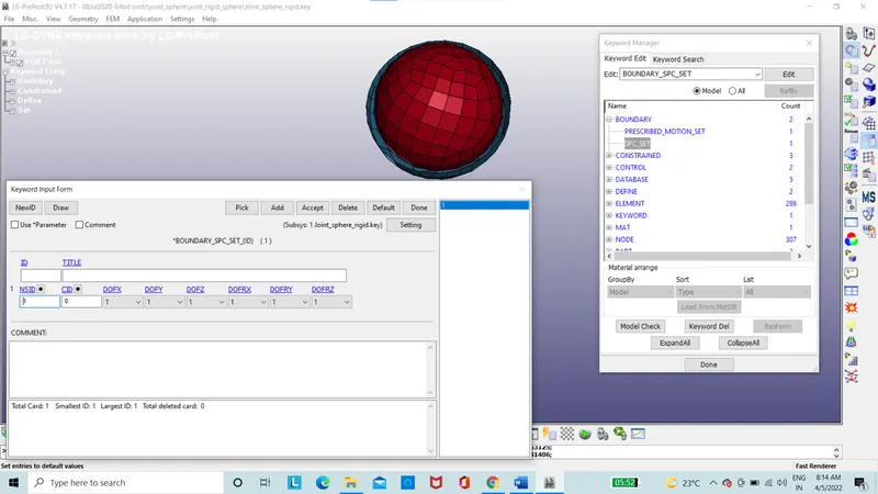
Figure 58: Boundary Spc set with Fixed condition
The Load curve is created using the define option.
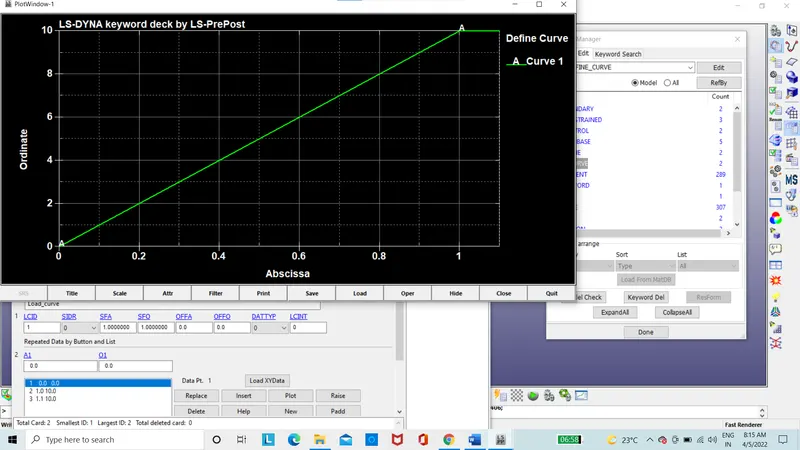
Figure 59: Load curve
The time step is created using the define option.
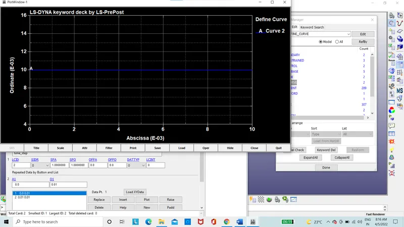
Figure 60: Time step curve
The boundary motion set is created with the displacement with LCID.
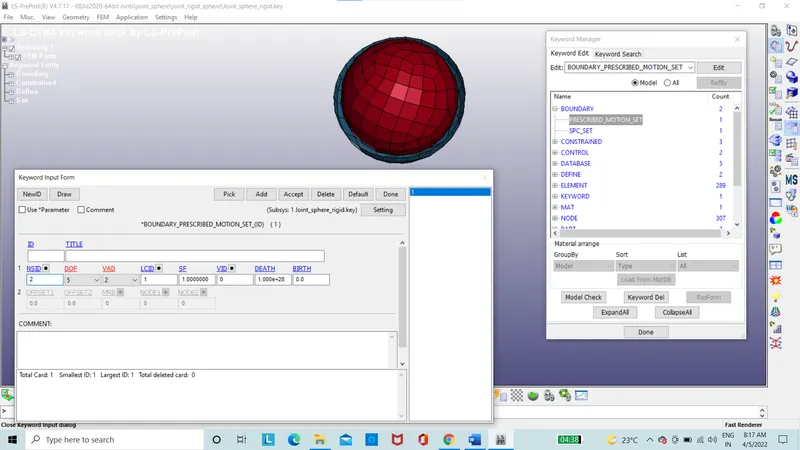
Figure 61: Boundary motion set
The Two nodes are created with node ID as 1000 and 1001.
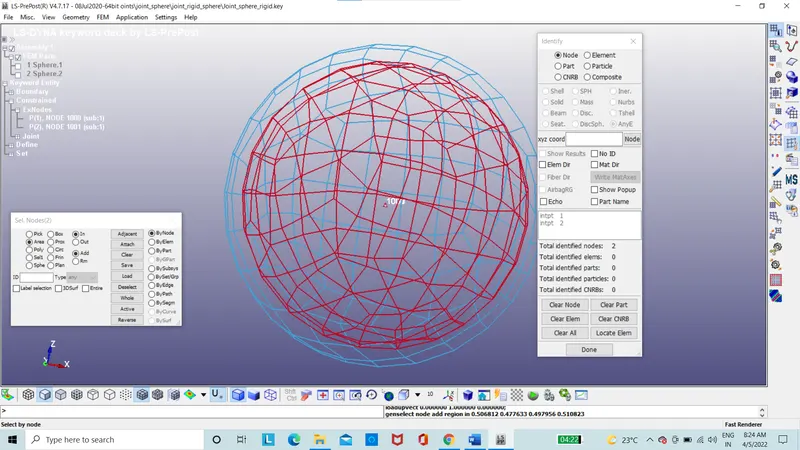
Figure 62: Nodes Coincident with each other
The constrained extra node set is created.
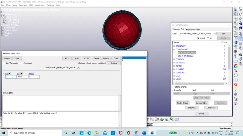
Figure 63: Constrained extra node for Part-1
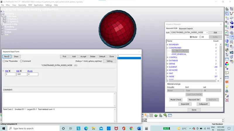
Figure 64: Constrained extra node for Part-2
The revolute joint is made using the constraint option.
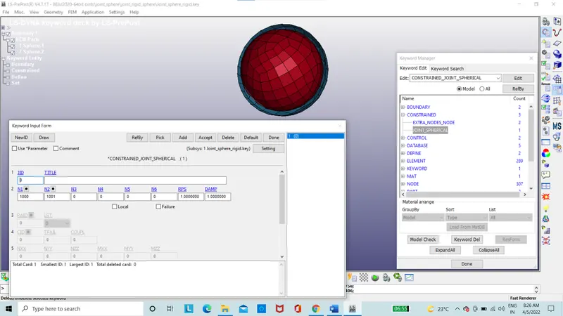
Figure 65: Constrained Spherical Joint
The time step card is used with LCTM input with time step curve.
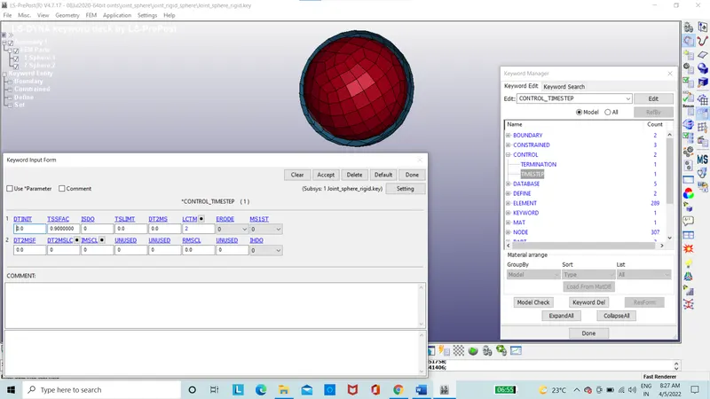
Figure 66: Time step card
The termination card is used.
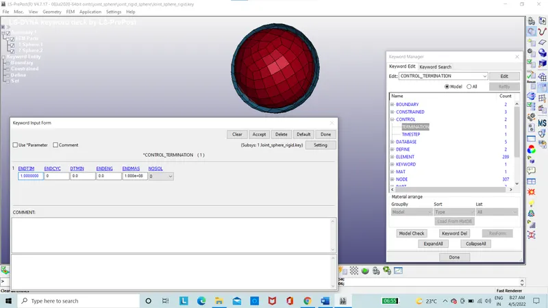
Figure 67: Termination card
The ASCII option is set using the database.
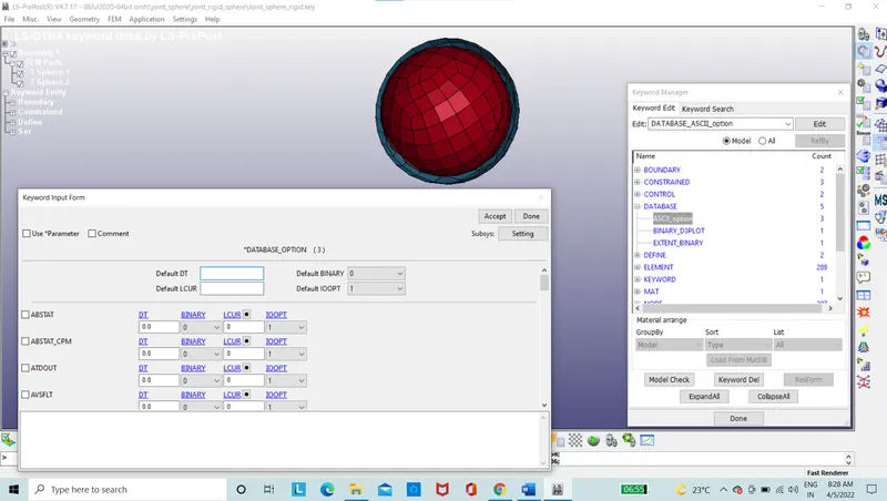
Figure 68: ASCII option.
The binary D3 plot is set using database.
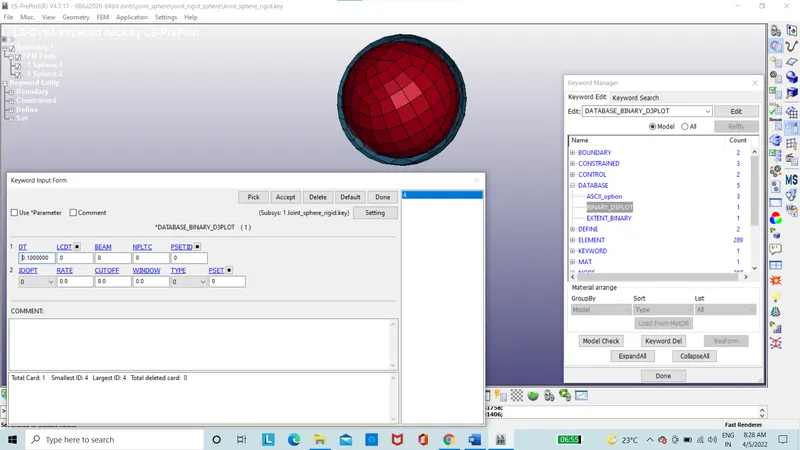
Figure 69: Binary D3plot
The Extent binary is set using the database.
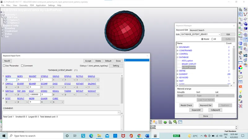
Figure 70: Extent Binary
The keyword File is saved and run.
Here, the two deformable bodies are considered by changing the material and replacing the constrain extra node with the Constrain Nodal rigid body (CNRB) and remaining cards would remain the same for the deformable spherical joint simulation.
The two bodies are considered to be rigid bodies with material properties card as MAT 24_piecewise Linear plasticity.
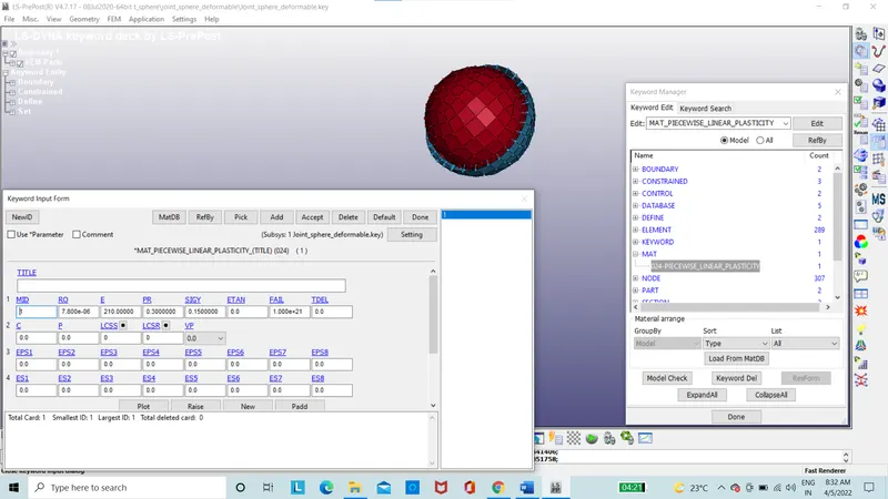
Figure 71: Mat 24_piecewise Linear plasticity
The Constrain Nodal rigid body (CNRB) is created by deleting the constrained extra node card.
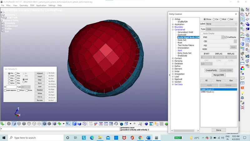
Figure 72: Constrain Nodal rigid body (CNRB)
The file is saved and run.
Results:
The revolute joint is simulated as rigid bodies with motion of rotation is obtained.
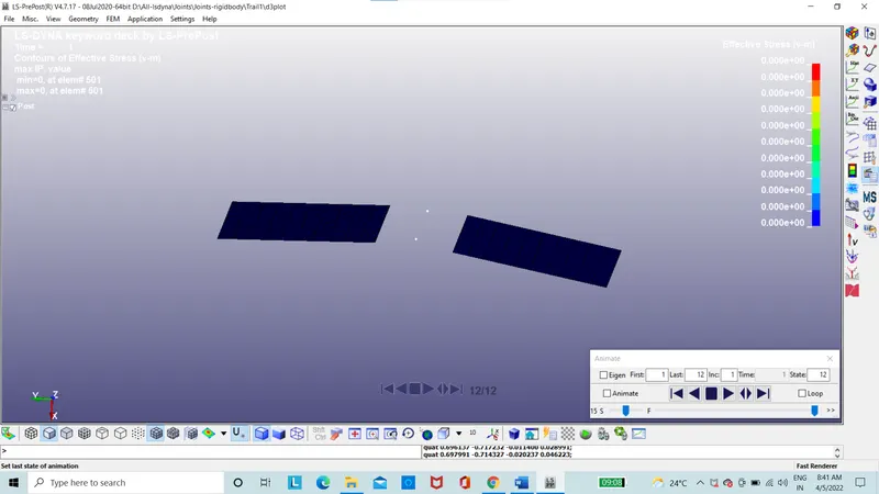
Figure 73: Revolute joint with Rigid bodies
The revolute joint is simulated as deformable bodies with motion of rotation is obtained.
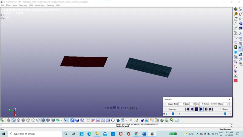
Figure 74: Revolute joint with deformable bodies
The joint forces of the Revolute joint with Rigid bodies.
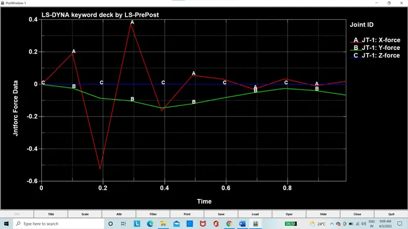
Figure 75: Joint forces of Revolute joint with Rigid bodies
The joint forces of the Revolute joint with deformable bodies.
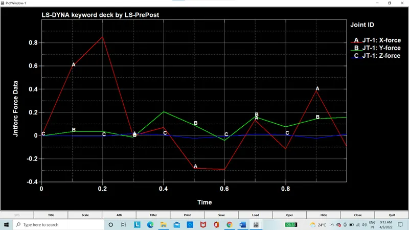
Figure 76: Joint forces of Revolute joint with deformable bodies
The joint moments of the Revolute joint with Rigid bodies.
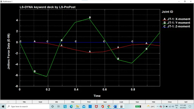
Figure 77: Joint moments of Revolute joint with Rigid bodies
The joint moments of the Revolute joint with deformable bodies.
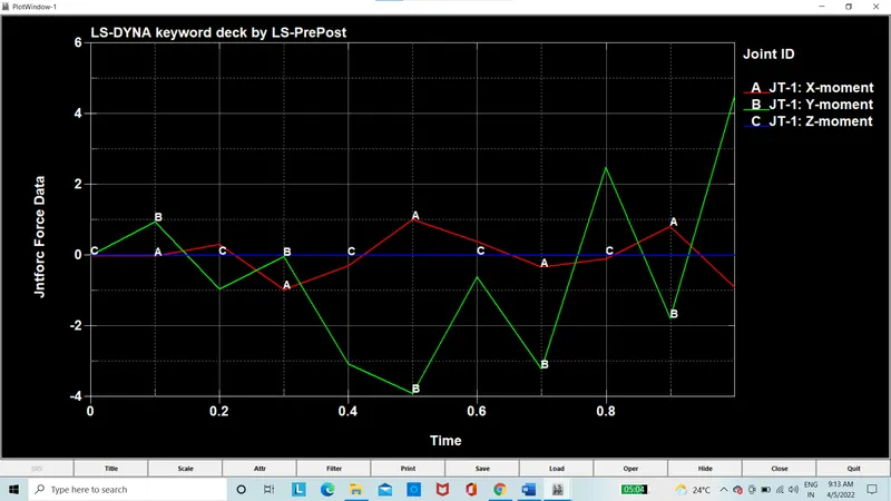
Figure 78: Joint moments of Revolute joint with deformable bodies
The cylindrical joint is simulated as rigid bodies with motion of rotation is obtained.
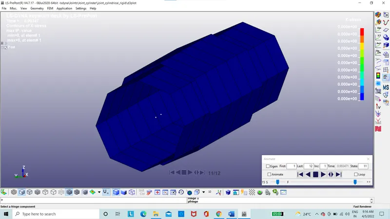
Figure 79: Cylindrical joint with Rigid bodies
The Cylindrical joint is simulated as deformable bodies with motion of rotation is obtained.
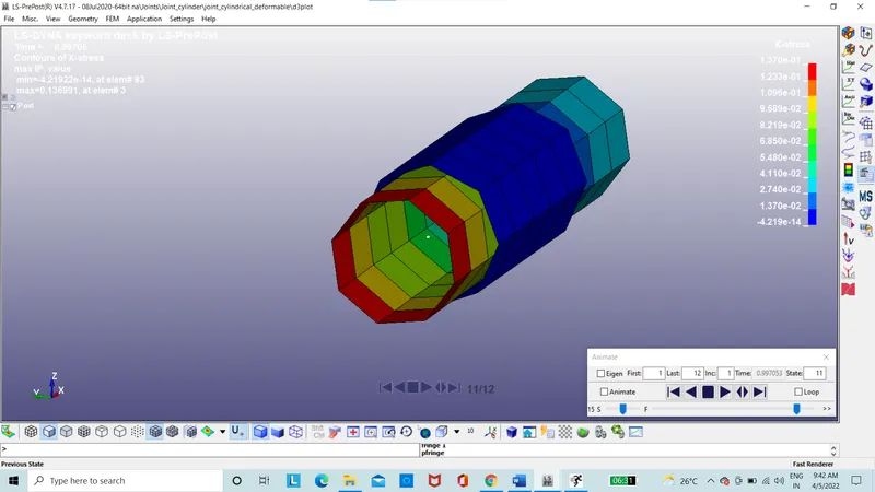
Figure 80: Cylindrical joint with deformable bodies
The joint forces of the cylindrical joint with Rigid bodies.
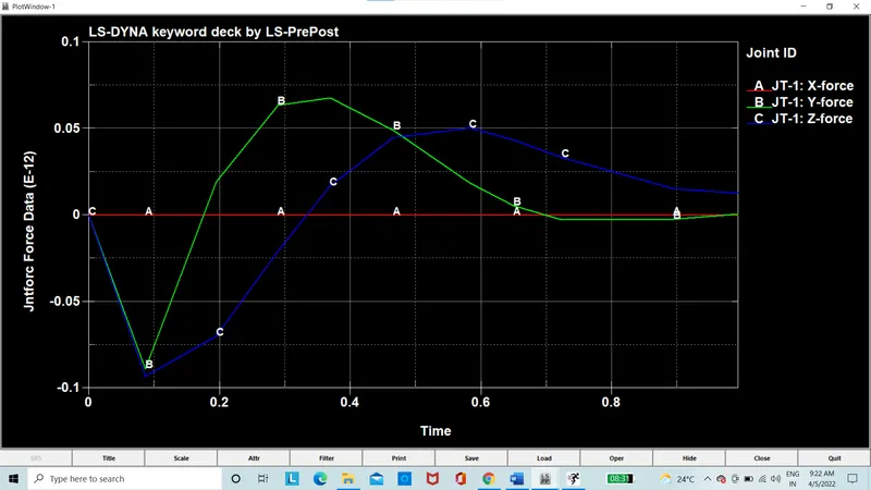
Figure 81: Joint forces of cylindrical joint with Rigid bodies
The joint forces of the cylindrical joint with deformable bodies.
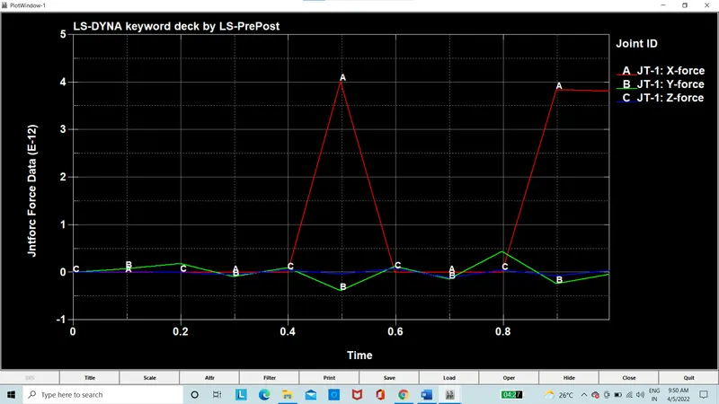
Figure 82: Joint forces of cylindrical joint with deformable bodies
The joint moments of the cylindrical joint with Rigid bodies.
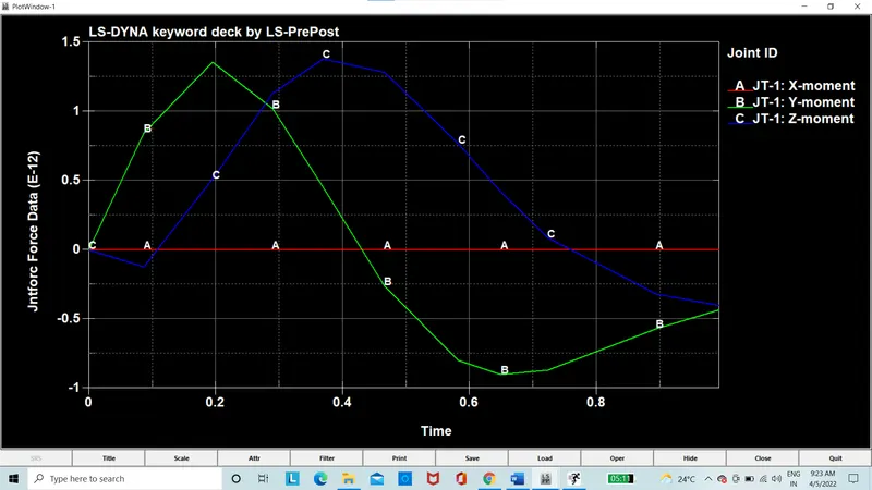
Figure 83: Joint moments of cylindrical joint with Rigid bodies
The joint moments of the cylindrical joint with deformable bodies.
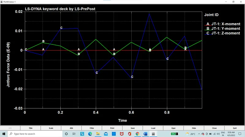
Figure 84: Joint moments of cylindrical joint with deformable bodies
The translational joint is simulated as rigid bodies with motion of rotation is obtained.
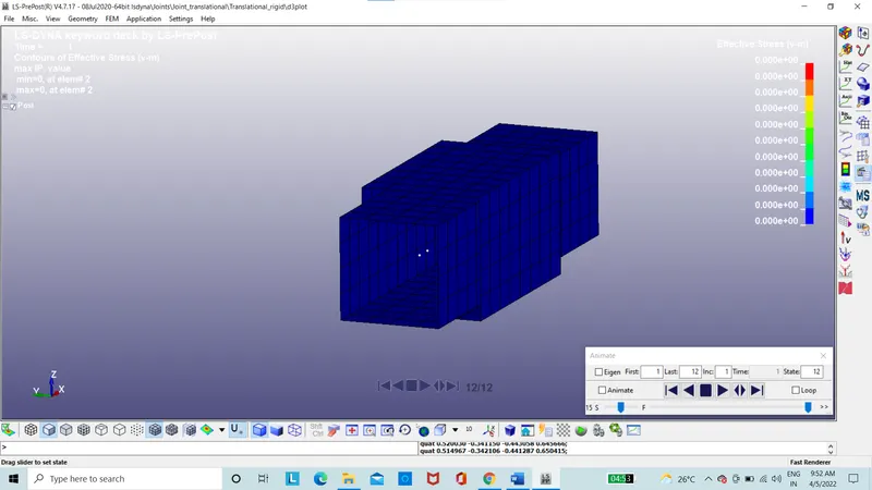
Figure 85: Translational joint with Rigid bodies
The translational joint is simulated as deformable bodies with motion of rotation is obtained.
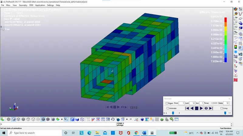
Figure 86: Translational joint with deformable bodies
The joint forces of the cylindrical joint with Rigid bodies.
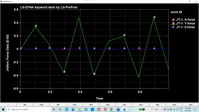
Figure 87: Joint forces of translational joint with Rigid bodies
The joint forces of the translational joint with deformable bodies.
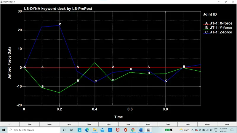
Figure 88: Joint forces of translational joint with deformable bodies
The joint moments of the translational joint with Rigid bodies.
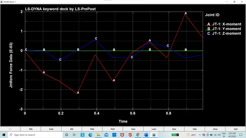
Figure 89: Joint moments of translational joint with Rigid bodies
The joint moments of the translational joint with deformable bodies.
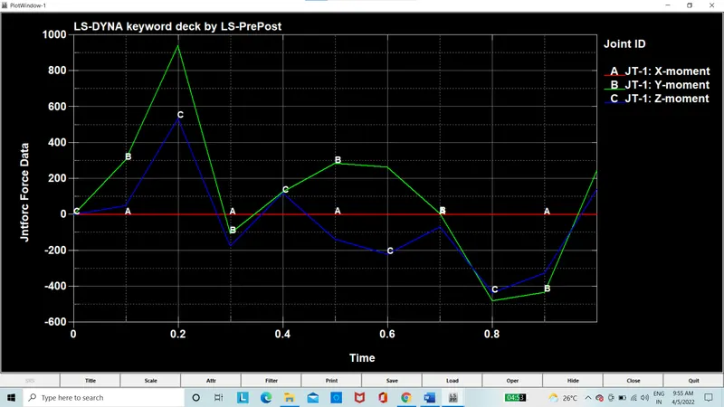
Figure 90: Joint moments of translational joint with deformable bodies
The Spherical joint is simulated as rigid bodies with motion of rotation is obtained.
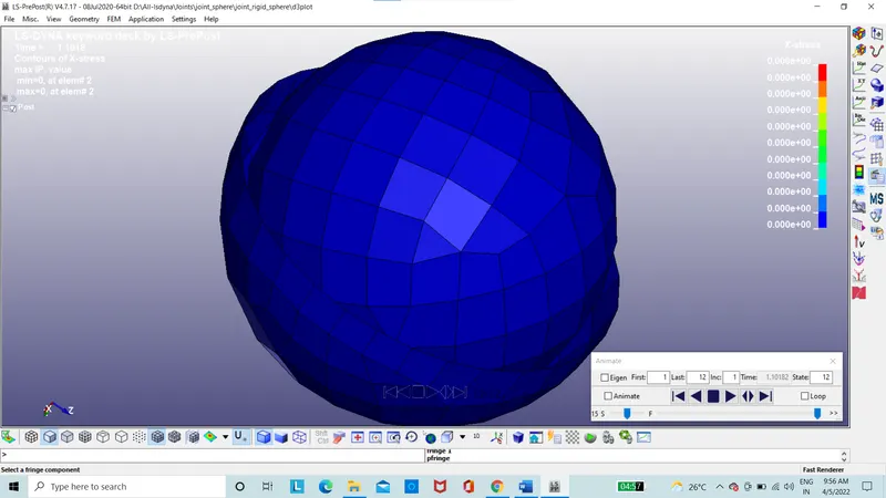
Figure 91: Spherical joint with Rigid bodies
The spherical joint is simulated as deformable bodies with motion of rotation is obtained.
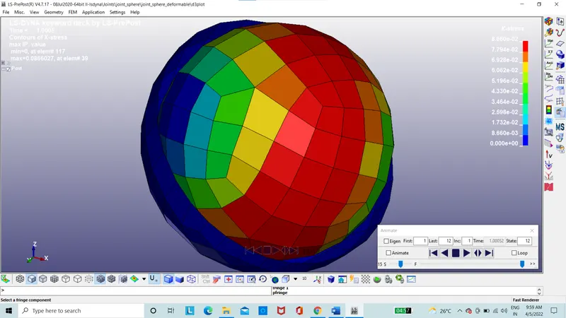
Figure 92: Spherical joint with deformable bodies
The joint forces of the spherical joint with Rigid bodies.
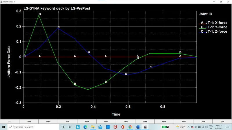
Figure 93: Joint forces of spherical joint with Rigid bodies
The joint forces of the spherical l joint with deformable bodies.
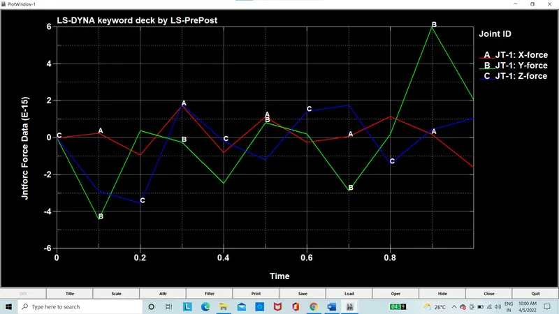
Figure 94: Joint forces of spherical joint with deformable bodies
The joint moments of the spherical joint with Rigid bodies.
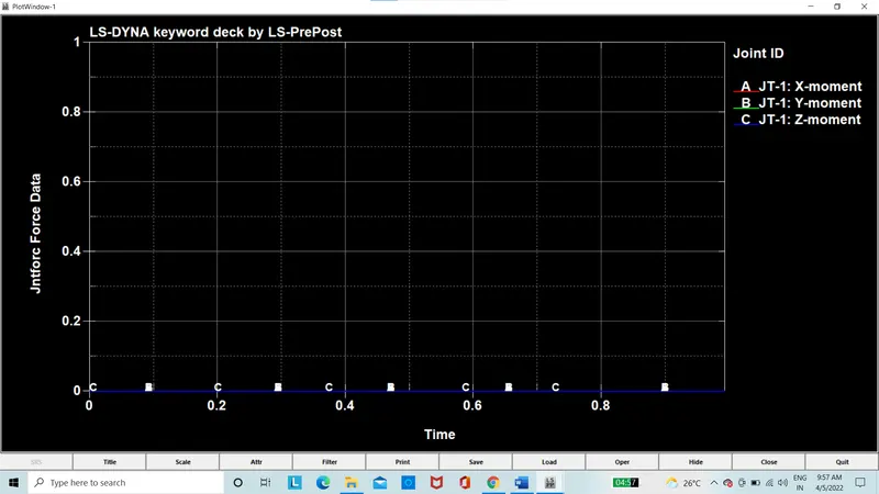
Figure 95: Joint moments of spherical joint with Rigid bodies
The joint moments of the spherical joint with deformable bodies.
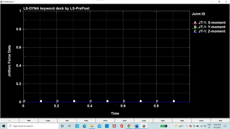
Figure 96: Joint moments of spherical joint with deformable bodies
Conclusion:
The revolute joint with rigid bodies and deformable bodies simulation is obtained, it is observed the motion produced is same with differences in the forces and moments produced. The cylindrical joint with rigid bodies and deformable bodies simulation is obtained, it is observed the motion produced is same with differences in the forces and moments produced. The translational joint with rigid bodies and deformable bodies simulation is obtained, it is observed the motion produced is same with differences in the forces and moments produced. The spherical joint with rigid bodies and deformable bodies simulation is obtained, it is observed the motion produced is same with differences in the forces and moments produced. The DOF free at rotation has not produced any moments as observed and where DOF free of translation motion the rection forces is not produced is observed.