Week - 4 - Crash Box Simulation
Aim: To create a simulation of crash box for impact test.
Objective: To crate a simulation of the crash box using the given mesh, the simulation of the crash with rigid wall and how it absorbs energy. The simulation helps understand the complex simulation by testing simple rectangular box with thickness 1.2mm and 1.5mm with initial and imposed velocity option and its combination to applied with differently for each simulation.
Procedure:
- The given model is downloaded and open in the Ls-dyna software by Ls-prepost.
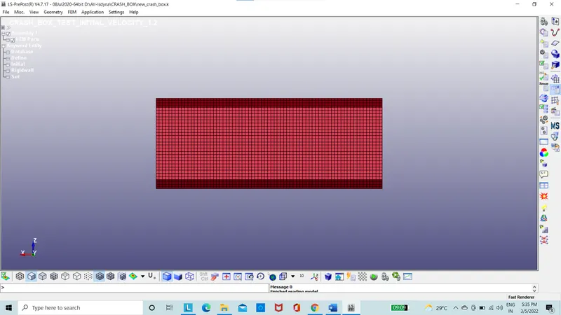
Figure 1: Crash box
- The model is given with “gm,mm,ms” dimensions, accordingly the values of the velocity, length etc are given.
- The section is taken as 1.2mm.
- The material is taken as steel in elastic limit input of density as 0.0078 gm/mm3 youngs modulus as 210000 g/mm.ms2 and possions ratio as 0.3.
- The part is input with material id and the section id.
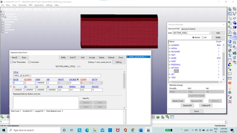
Figure 2: Section id
- The rigid wall was created at a distance of 15mm from the edge of the wall.
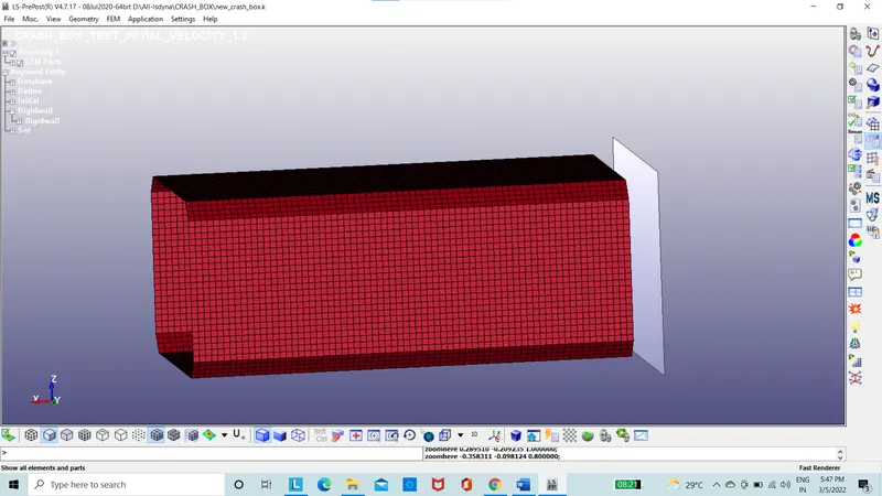
Figure 3: Rigid wall
- The initial velocity is input into the node set which is created on the box.
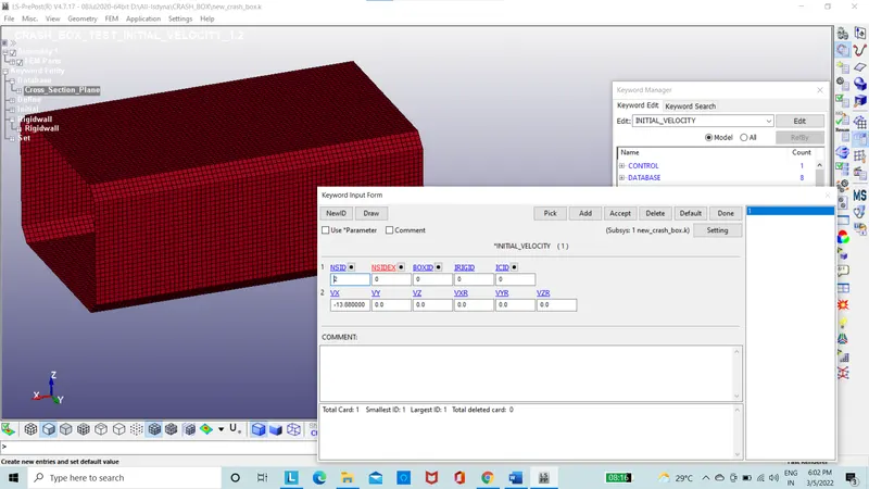
Figure 4: Initial velocity Input
- Section place is created on the middle of the crash box.
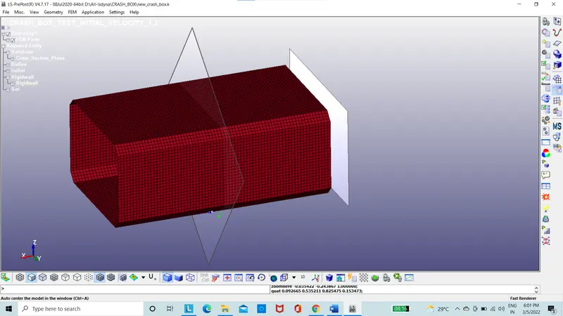
Figure 5: Section plane
- The database is set for ASCII with GLSTAT,MATSUM,GLEOUT,RCFORC.
- Binary database as D3 plot.
- The termination time is set as 2mm.
- The input file is run on Ls-run.
- The command file is run.
- The result file is obtained.
- The result of stress, energies etc are taken into consideration.
- The same file is used to create another simulation with imposed velocity with elasto plastic material property of steel with thickness 1.5mm.
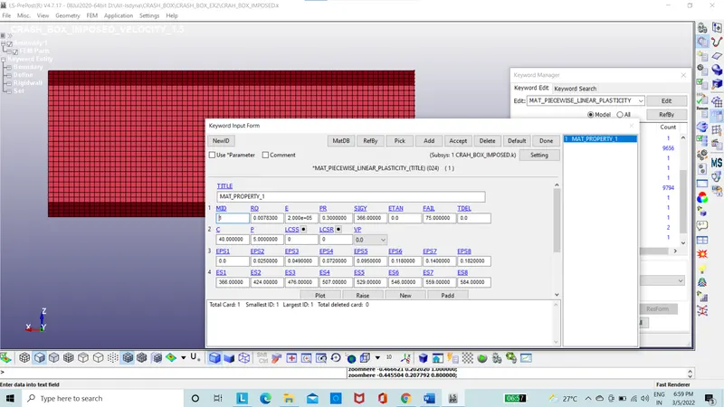
Figure 6: Model with Material property
- The imposed velocity is applied on the CNRB nodal rigid body master node.
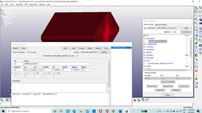
Figure 7: Model with CNRB
- The database is set for ASCII with GLSTAT,MATSUM,GLEOUT,RCFORC.
- Binary database as D3 plot.
- The termination time is set as 2mm.
- The input file is run on Ls-run.
- The command file is run.
- The result file is obtained.
- The same file is used to create another simulation with elastic material property of steel with thickness 1.5mm.
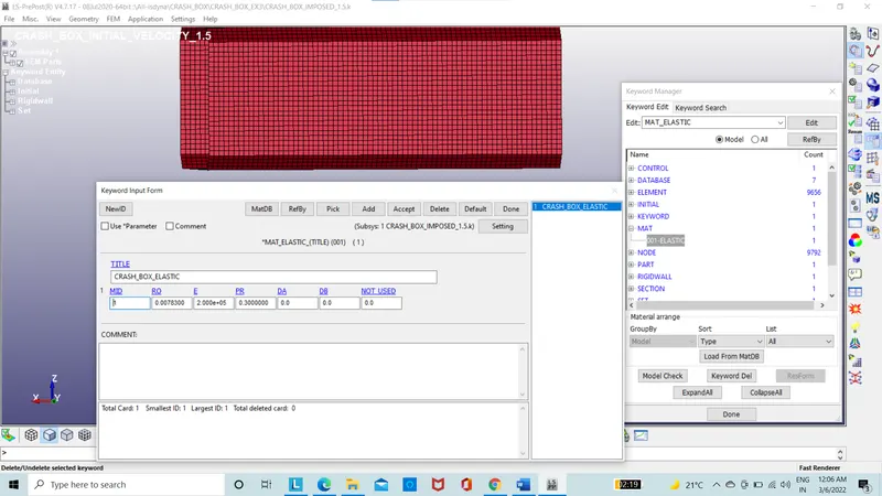
Figure 8: Model with Material property
- The initial velocity is applied.
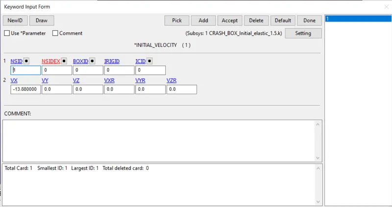
Figure 7: Model with initial velocity
- The database is set for ASCII with GLSTAT,MATSUM,GLEOUT,RCFORC.
- Binary database as D3 plot.
- The termination time is set as 2mm.
- The input file is run on Ls-run.
- The command file is run.
- The result file is obtained.
- The same file is used to create another simulation with imposed velocity and elastic material property of steel with thickness 1.2mm.
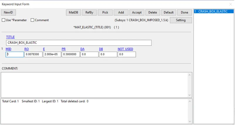
Figure 6: Model with Material property
- The imposed velocity is applied on the CNRB nodal rigid body master node.
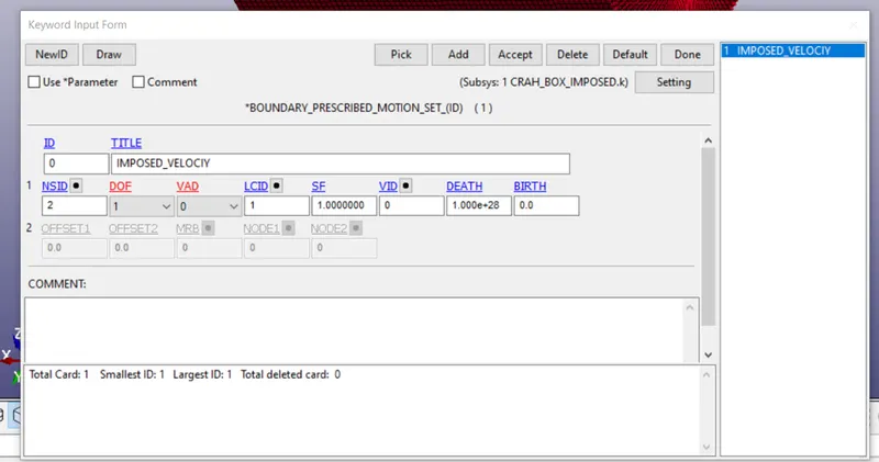
Figure 7: Model with CNRB
- The database is set for ASCII with GLSTAT,MATSUM,GLEOUT,RCFORC.
- Binary database as D3 plot.
- The termination time is set as 2mm.
- The input file is run on Ls-run.
- The command file is run.
- The result file is obtained.
- The same file is used to create another simulation with imposed velocity with elastic material property of steel with thickness 1.5mm.
Figure 6: Model with Material property
- The imposed velocity is applied on the CNRB nodal rigid body master node.
Figure 7: Model with CNRB
- The database is set for ASCII with GLSTAT,MATSUM,GLEOUT,RCFORC.
- Binary database as D3 plot.
- The termination time is set as 2mm.
- The input file is run on Ls-run.
- The command file is run.
- The result file is obtained.
- The same file is used to create another simulation with elasto plastic material property of steel with thickness 1.2mm.
Figure 6: Model with Material property
- The initial velocity is applied.
Figure 7: Model with initial velocity
- The database is set for ASCII with GLSTAT,MATSUM,GLEOUT,RCFORC.
- Binary database as D3 plot.
- The termination time is set as 2mm.
- The input file is run on Ls-run.
- The command file is run.
- The result file is obtained.
Results:
The cross-sectional force along the length of the crash box.
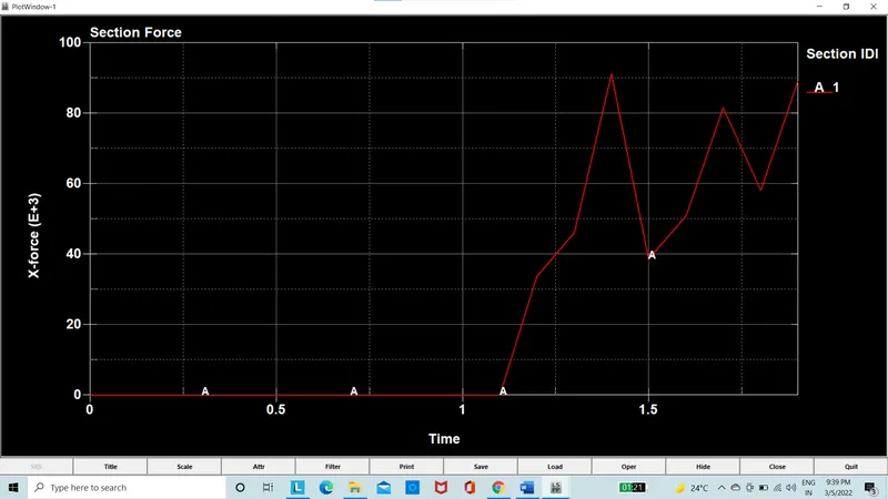
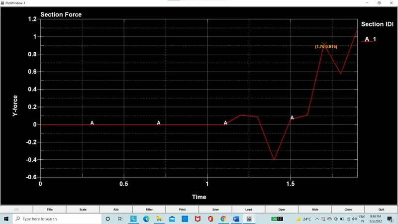
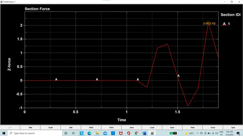
Figure 8: the sectional forces along X, Y and Z direction are plotted for crash box with 1.2mm thickness
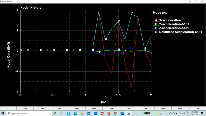
Figure 9: Acceleration for crash box 1.2mm thickness
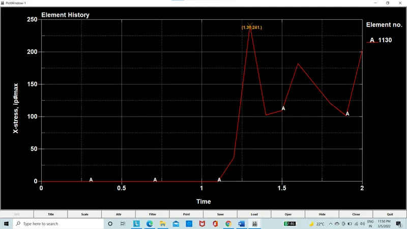
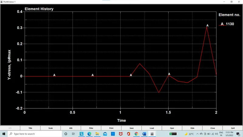
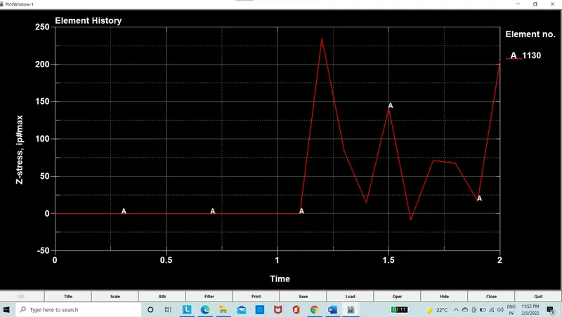
Figure 10: Maximum directional stress
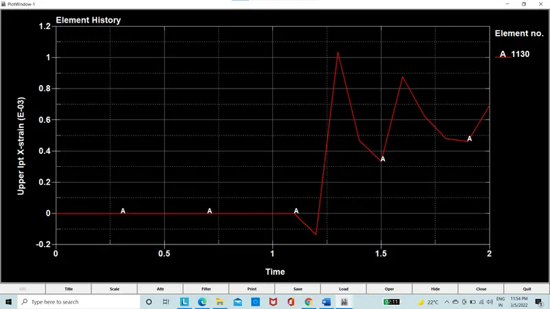
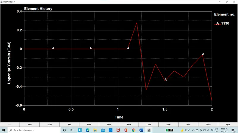
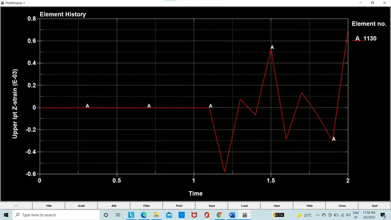
Figure 11: Maximum Directional Strain
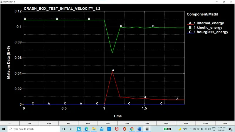
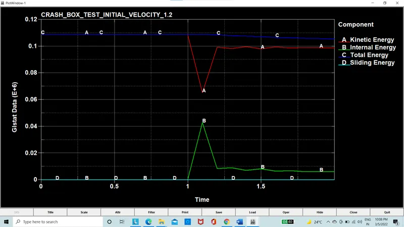
Figure 12: plot of energies for crash box 1.2mm thickness
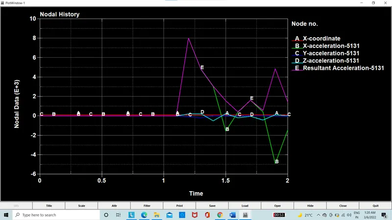
Figure 13: Comparison of Accelerations of 1.2mm and 1.5mm Crash Box respectively
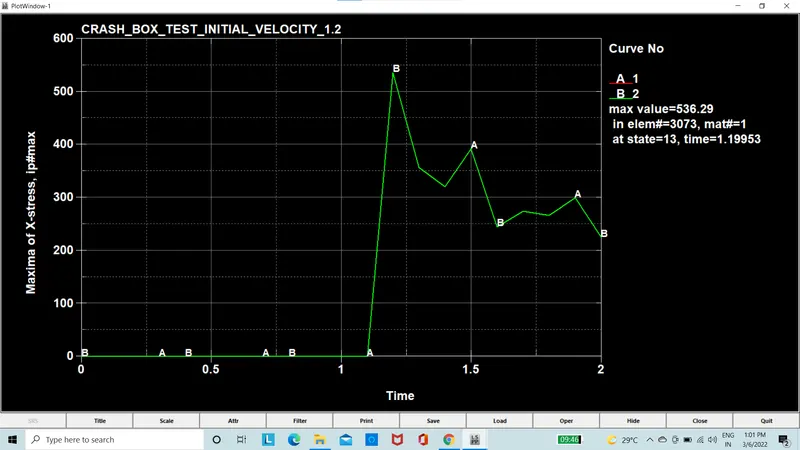
Figure 14(a): X-directional stress plot of crash box 1.2mm
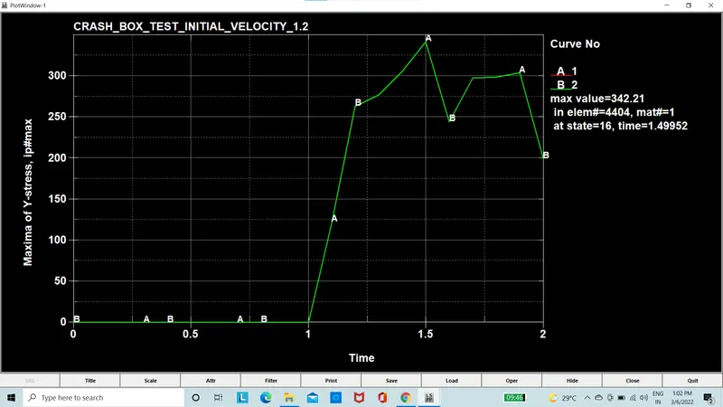
Figure 14(b): y-directional stress plot of crash box 1.2mm
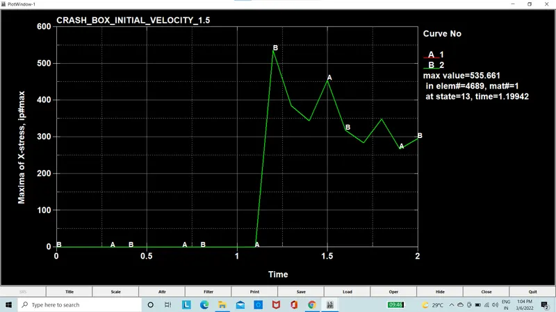
Figure 14(c): x-directional stress plot of crash box 1.5mm
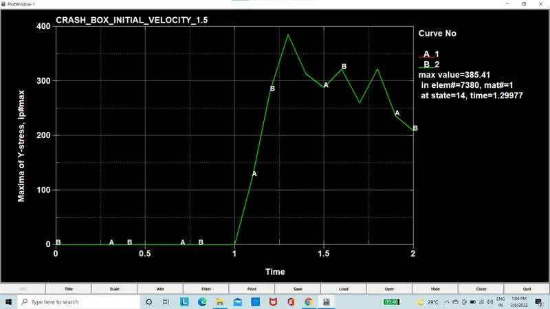
Figure 14(d): y-directional stress plot of crash box 1.5mm
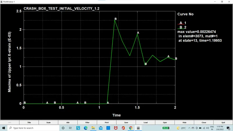
Figure 14(e): X-directional strain plot of crash box 1.2mm
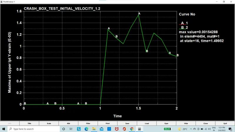
Figure 14(f): y-directional strain plot of crash box 1.2mm
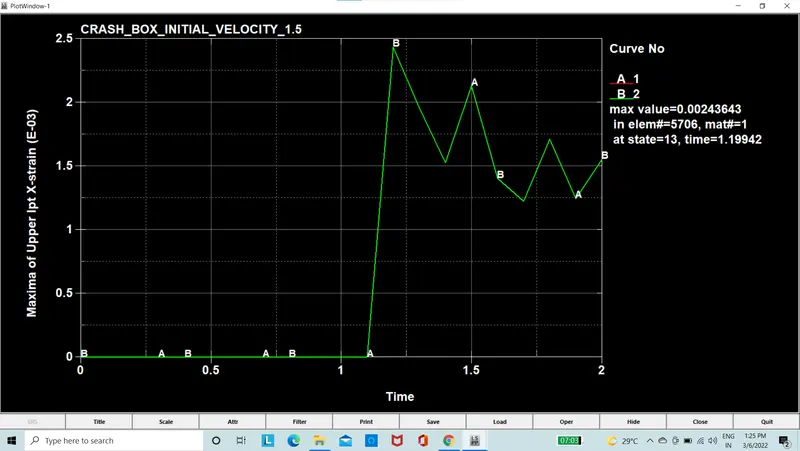
Figure 14(g): X-directional strain plot of crash box 1.5mm
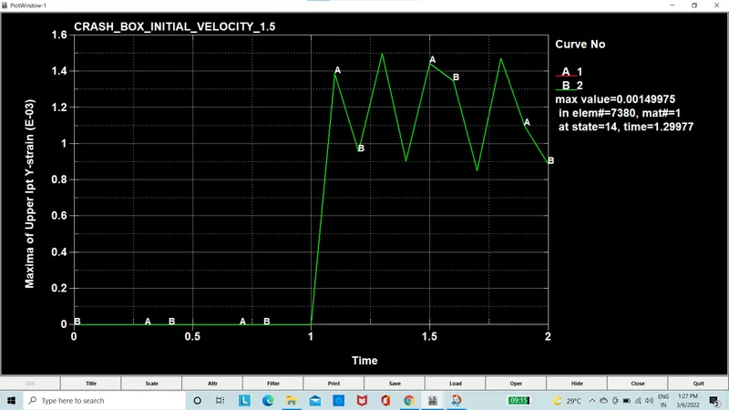
Figure 14(g): y-directional strain plot of crash box 1.5mm
Figure 14: Comparison of Stress/strain Plot of 1.2mm and 1.5mm Crash Box in X and Y direction
conclusion:
The crash box 1.2mm and 1.5mm is having slight change in energy, stress and strain.
the crash box 1.5mm absorbs more energy than 1.2mm and the stresses are little less in 1.5 compared to1.2mm
the combination of imposed velocity and initial velocity with elastic and elasto plastic material are created and uploaded with result and input files.
Note: Animation, result files are attached.