Week - 9 Material Modeling from Raw Data
Aim: To material model from the raw data given by using the material card of MAT-024_Linear_piecewise_plasticity card in Ls-dyna
Objective:
To model a material from the raw data given in the form of image to be extracted using the data digitizer and clean up the data, plot the graph to check that the data is matching the original data. The data here should be proper and all the calculation needs to be in the form “Kg-mm-ms” dimension system. The said material model is now validated using the data in the dog bone specimen for cross verification by simulating the tensile test. The data is validated by matching the output data with the original data.
Procedure:
The data obtained from the lab test is provided as in the form of image and is extracted from the data digitizer software.
The data of the graphite iron casting is obtained in the excel sheet.
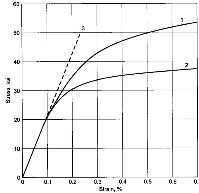
Figure 1: Raw data in Image format
The data point obtained is for the curve 1 and the MAT-024_Linear_piecewise_plasticity card is taken into consideration. The data point extracted is stress(ksi) in X-axis is (0,0.7) and strain% Y-axis is (0,60).
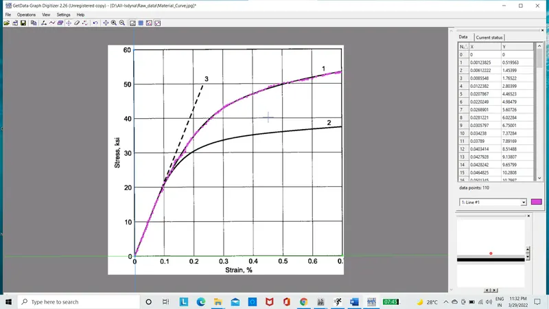
Figure 2: Get data digitizer used for data point extraction
The data points obtain will be exported and cleaned up in the form of excel sheet and with be saved in the CSV format so that it works properly in the Ls-dyna software.
The true stress and true strain% in the excel sheet is taken into consideration
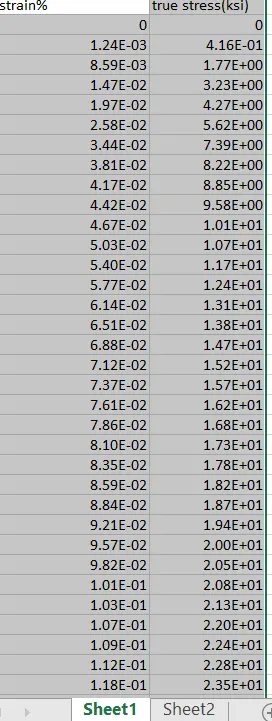
Figure 3: excel sheet with true stress and strain% data
The data is now plotted with true stress/strain% graph
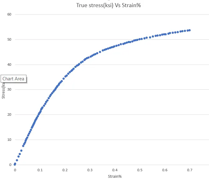
Figure 4: True stress VS Strain% graph
This is to make sure that the given raw data matches with the obtained data points from the get data digitizer is exactly the same plot. Therefore, have to clean up the data since the Ls-dyna accepts only the monotonically increasing curves.
The value obtained are of true stress and strain %, therefore strain % is converted to true strain by dividing strain % by 100.

Figure 5: True strain excel sheet value.
The true stress and strain is obtained, however it is to be converted to “Kg-mm-ms” dimension. The stress which is in the Kilo pound per square inches is converted to pa. 1Ksi is equal to 6894760Pa. Therefore, multiplying the stress in ksi into pa.

Figure 6: True stress(pa) excel sheet value.
The true stress(pa) is to be in the “kg-mm-ms” dimension; hence a conversion factor of 10^-9 conversation factor is used to get effective stress.

Figure 7: Effective stress
The true stress Vs Strain graph is obtained to determine the yield strength the material.
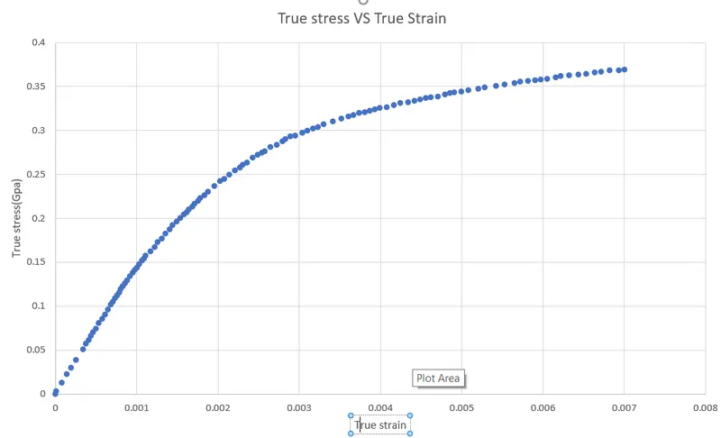
Figure 8: True stress Vs true strain
Young’s modulus is given in the data to be 20.9E+06 psi, therefore converting to pascal 20.9E+6 Psi= 144100427427 pascal, it’s the multiplied with conversion factor as 10^-9 to be in “Kg-mm-ms”. Young’s modulus= 144.1 Gpa
The effective plastic strain is calculated using the formulae,
Effective plastic strain = Total true strain – (total true stress/Young’s modulus)
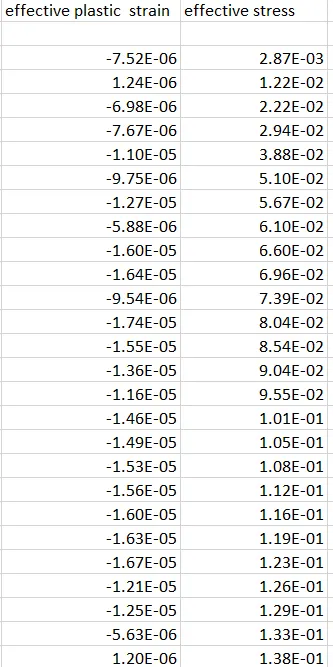
Figure 9: Effective stress and effective plastic strain data
The effective stress VS effective strain graph is plotted to find the stress/strain curve
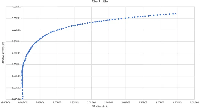
Figure 10: Effective stress and effective plastic strain graph
From the graph we can see the non-linearity starts at 1.5E-1 Gpa, therefore we can consider that as the yield point and the curve after the yield point is taken into consideration.
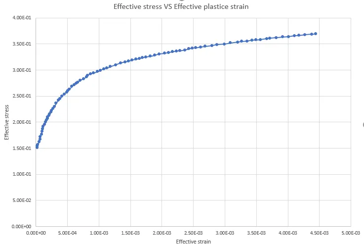
Figure 11: Effective Plastic Region Graph
The data obtained by this graph is taken into account to be considered as the LCSS as material curve in the dog bone specimen for tensile test in Ls-dyna.
The dog bone specimen is opened in the Ls-dyna.
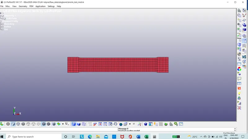
Figure 12: the dog bone specimen
The material curve is defined using the define curve option
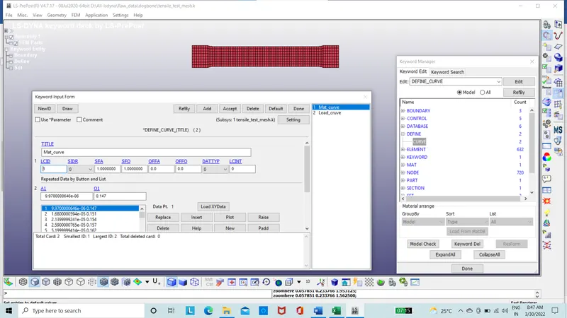
Figure 13: The material curve
The section of the dog bone with a thickness of 2mm is taken.
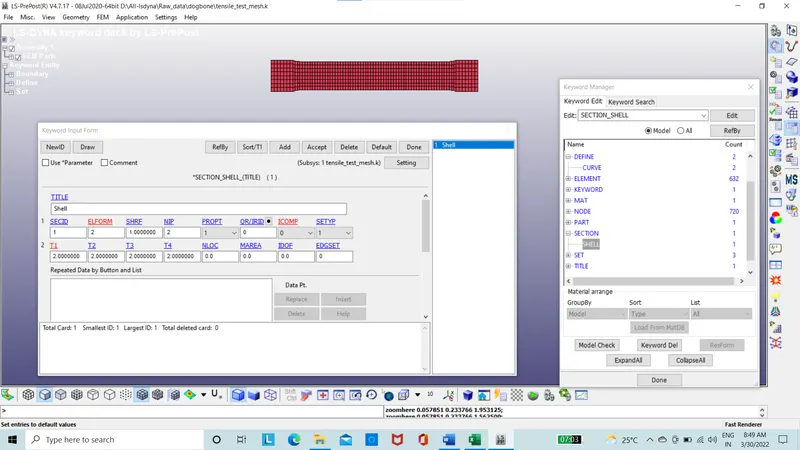
Figure 14: The section card
The Material card of MAT-024_Linear_piecewise_plasticity is taken
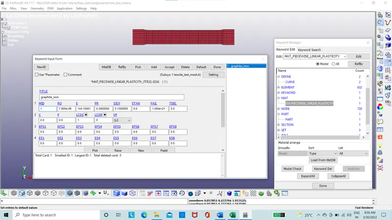
Figure 15: The material card
The load curve is defined to apply load
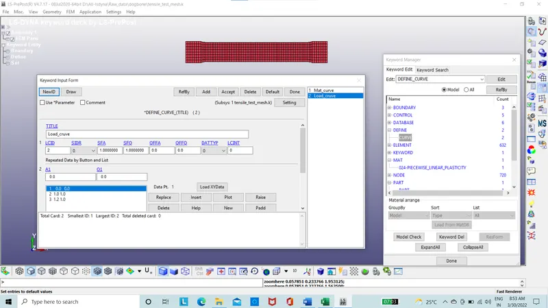
Figure 16: The load curve
The boundary spc set is created to constrain the model in all direction
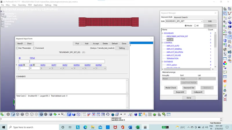
Figure 17: The Boundary spc
The boundary spc set is created to constrain the model in Y direction
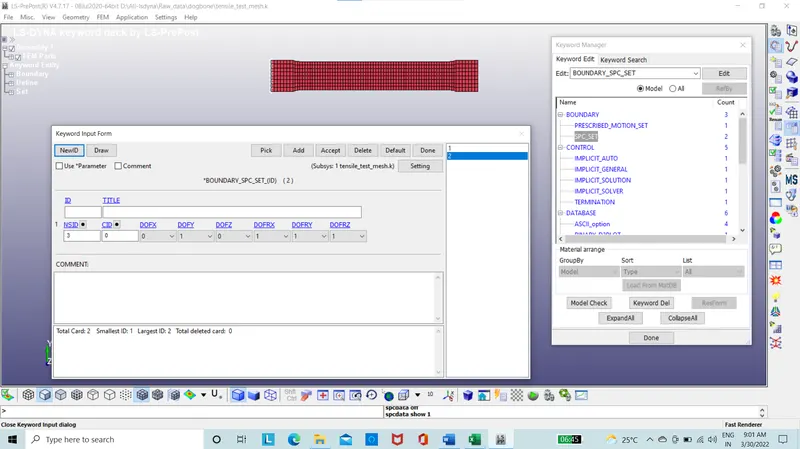
Figure 18: The Boundary spc in y-direction
The displacement is applied to the model using the prescribed motion set
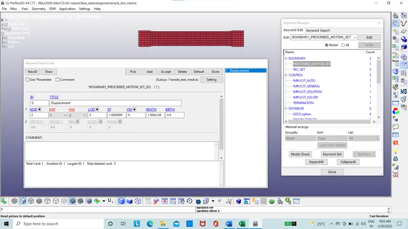
Figure 19: The prescribed motion set card
The model is better run by the implicit analysis since it’s a tensile test. The implicit analysis cards are introduced using the control option.
The implicit auto card is used
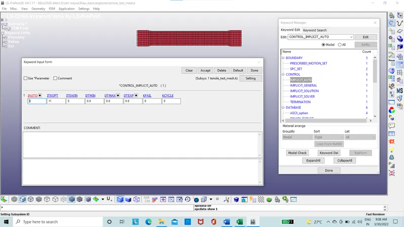
Figure 20: The implicit auto card
The implicit general card is used
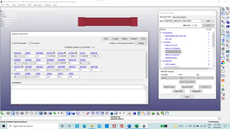
Figure 21: The implicit general card
The implicit solution card is used
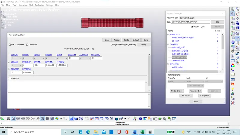
Figure 22: The implicit solution card
The implicit solver card is used
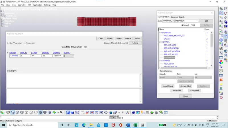
Figure 23: The implicit solver card
The termination time is introduced
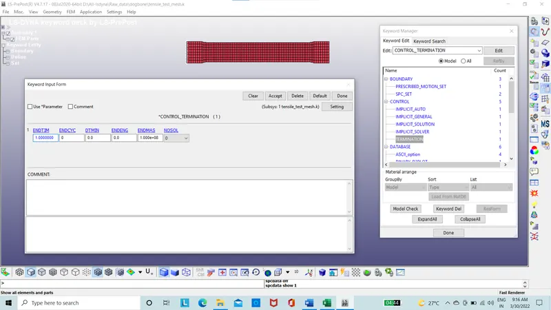
Figure 24: The termination time card
The database control card with ASCII option, D3PLOT, Extent binary where strflg is set to 1 for the plastic strain results to be displaced is applied
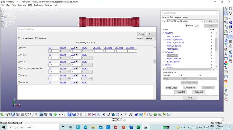
Figure 25: The ASCII option card
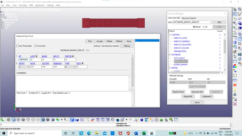
Figure 26: The Binary D3PLOT card
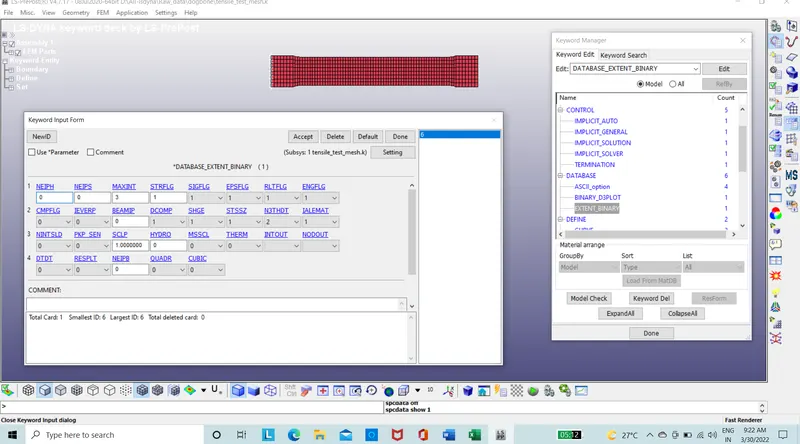
Figure 27: The Extent binary card
The Keyword is saved and the file run.
Results:
The stress contour is plotted for the dog bone specimen which is von-misses stress which also known as the equivalent stress considered as effective stress
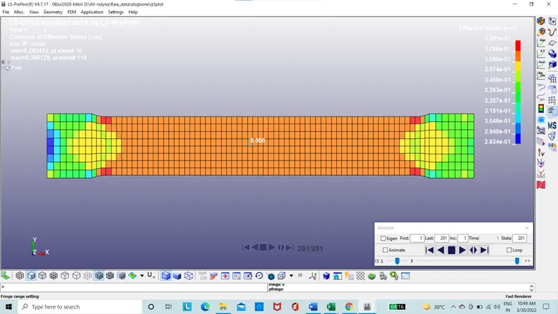
Figure 28: Stress contour plot
The stress produced at the specimen is 0.389 Gpa from the observation.
The effective plastic strain contour is plotted for the dog bone specimen.
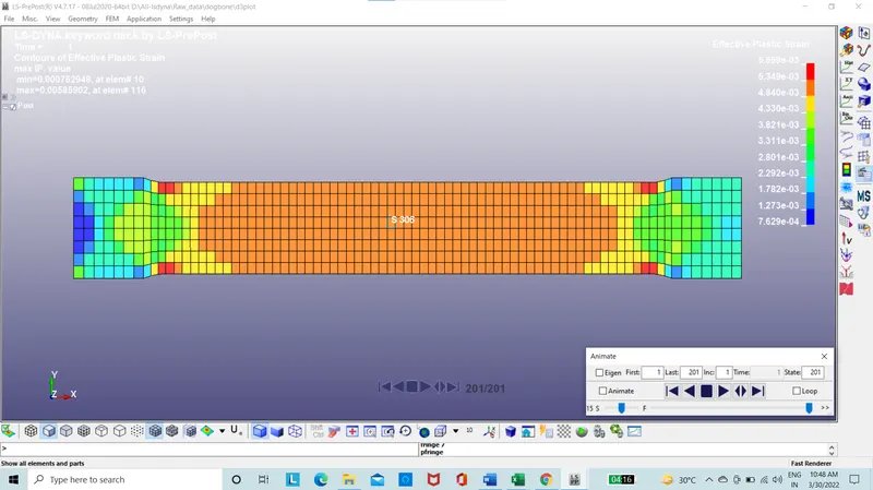
Figure 29: Effective plastic strain contour
The strain obtained from the contour is 0.00585.
The effective stress vs time curve is obtained from the element 306 from History graph
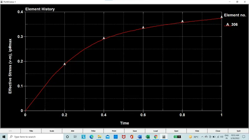
Figure 30: Effective stress Vs time curve graph
The effective plastic strain vs time curve is obtained from the element 306 from History graph
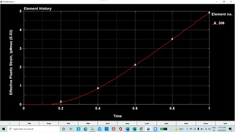
Figure 31: Effective strain Vs time curve graph
The effective stress and effective plastic strain curves are saved in the form of excel data in CSV format and effective stress Vs effective plastic strain curve is obtained.
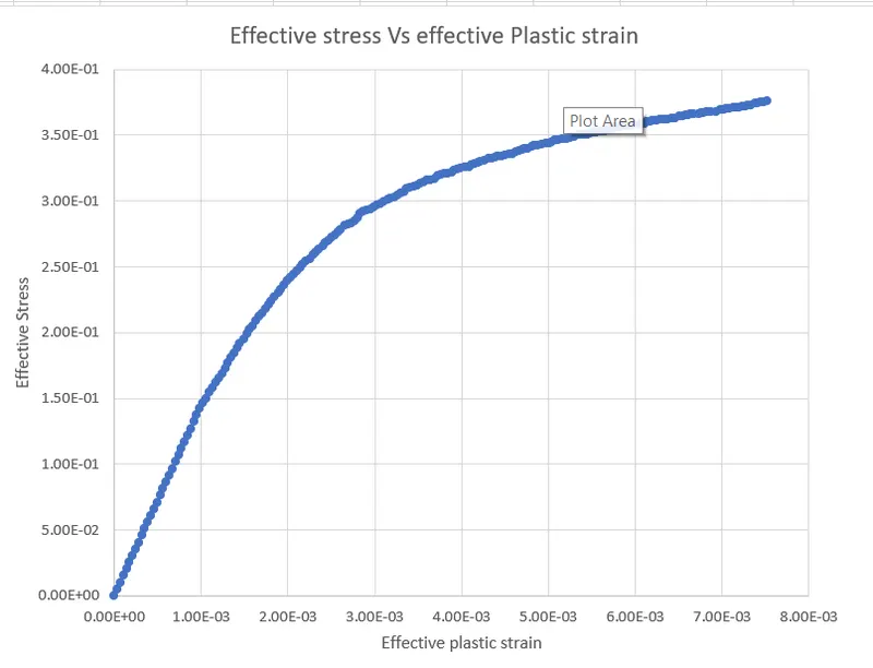
Figure 32: Effective stress Vs effective plastic strain curve graph from dog bone
This curve of the effective stress Vs effective plastic strain curve graph from the dog bone specimen is compared with given raw material data is compared.
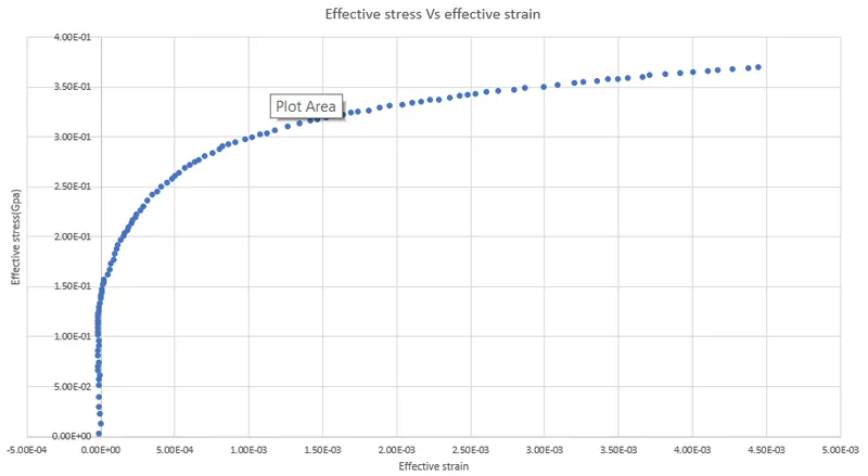
Figure 33: effective stress Vs effective plastic strain curve graph of raw material data
The True stress Vs true strain of the raw data and the effective stress Vs effective plastic strain is overlapped on each other to compare the curve.
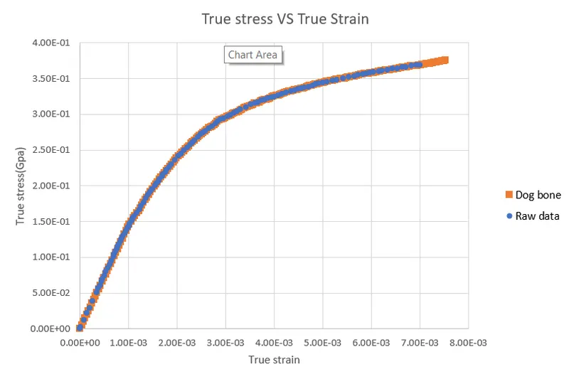
Figure 34: True stress Vs True strain curve overlapping effective stress Vs effective plastic
The True stress Vs True strain curve overlapping the effective stress Vs effective plastic strain curve graph, therefore can be concluded to be validated.
Conclusion:
The material modelling from the raw data is cleaned up, converted to effective stress and effective plastic strain. The effective stress Vs effective plastic strain curve is the obtained from the dog bone specimen and this is compared with the raw data given. The true stress Vs true strain curve and effective stress Vs effective plastic strain curve is same by comparing with dog bone specimen and the raw data provided by overlapping on each other. Therefore, the validation of the material modeling of the raw data with the dog bone specimen is completed.