Week - 8 Mass Scaling
Aim: The Mass scaling of the given model is done to reduce the run time and ensure the stability of the model and comparing the run time of the model by implicit and explicit method.
Objective: The given model is subjected to explicit analysis modeling and is run without the timestep control to know the time and mass scaling, then with the timestep with mass scaling is run and time reduction is noted down. The number of iterations is done, increasing the mass scaling is by increasing the DT2MS value and comparing the time required to run each of these simulation times is noted down. Then Histogram of the values are plotted with runtime with the mass scaling.
Mass scaling:
The mass scaling is done to increase the time step by adding the artificial mass to the element of the smallest element of the system, the time step is measure by the courant’s stability criteria, t=Le/c, where Le represents the characteristics length of the element, c represents the speed of sound. Where, c= Ls-dyna allows two different types of mass scaling using the DT2MS parameters from “Control timestep” with the default set to no mass scaling. When DT2MS is less than zero, the mass is added to each element whose timestep is below abs (DT2MS) such that the element’s updated DT is equal to abs (DT2MS). When DT2MS is greater than Zero, LS-dyna adds mass to the elements whose DT is below abs(DT2MS) and “removes” mass from elements whose DT is greater than Zero.
Procedure:
The given model is downloaded and the model is opened in the Ls-dyna software.
The model is run as Explicit Analysis to find the default timestep of DT2MS value by deleting the timestep in control option.
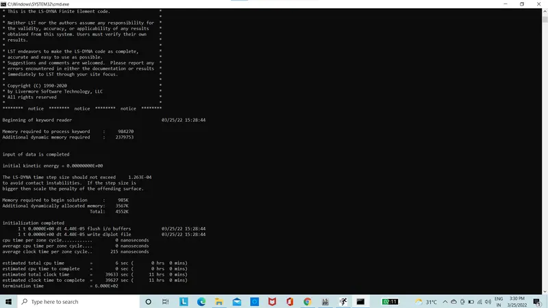
Figure 1: Default DT2MS value
The model is now added with mass by giving the value of TSSFAC=0.9 and DT2MS=-5.5E-5
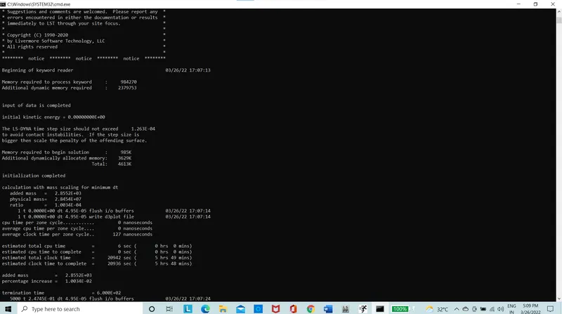
Figure 2: Model with DT2MS as -5.5E-5
The model is now added with mass by giving the value of TSSFAC=0.9 and DT2MS=-6.5E-5
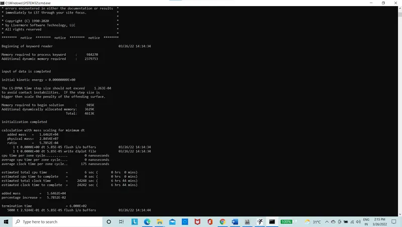
Figure 3: Model with DT2MS as -6.5E-5
The model is now added with mass by giving the value of TSSFAC=0.9 and DT2MS=-7.5E-5
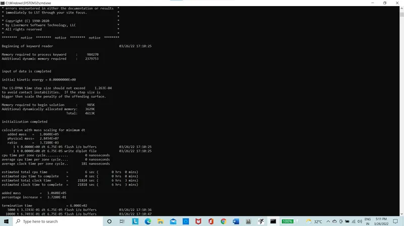
Figure 4: Model with DT2MS as -7.5E-5
The model is now added with mass by giving the value of TSSFAC=0.9 and DT2MS=-8.5E-5
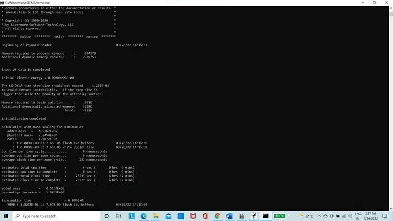
Figure 5: Model with DT2MS as -8.5E-5
The model is now added with mass by giving the value of TSSFAC=0.9 and DT2MS=-9.5E-5
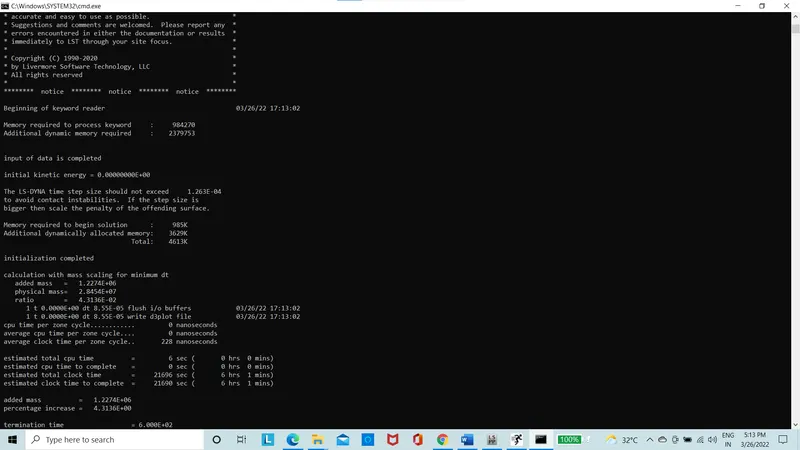
Figure 6: Model with DT2MS as -9.5E-5
The model is now added with mass by giving the value of TSSFAC=0.9 and DT2MS=-1.03E-4
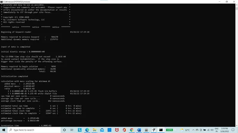
Figure 7: Model with DT2MS as -1.03E-4
The value of DT2MS is not further increased as the value of percentage increased will increase more than the hard limit of 8%, therefore will stop the iteration till DT2MS is -1.03E-4.
Now further the Explicit Analysis is carried out with change in TSSFAC with same value of DT2MS to compare the results.
The model is now added with mass by giving the value of TSSFAC=0.8 and DT2MS=-5.5E-5
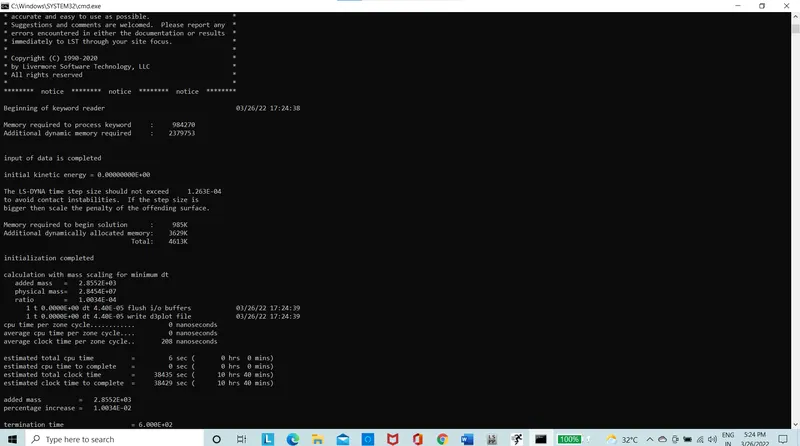
Figure 8: Model with DT2MS as -5.5E-5
The model is now added with mass by giving the value of TSSFAC=0.8 and DT2MS=-6.5E-5
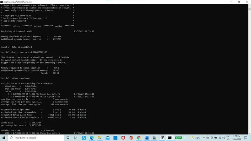
Figure 9: Model with DT2MS as -6.5E-5
The model is now added with mass by giving the value of TSSFAC=0.8 and DT2MS=-7.5E-5
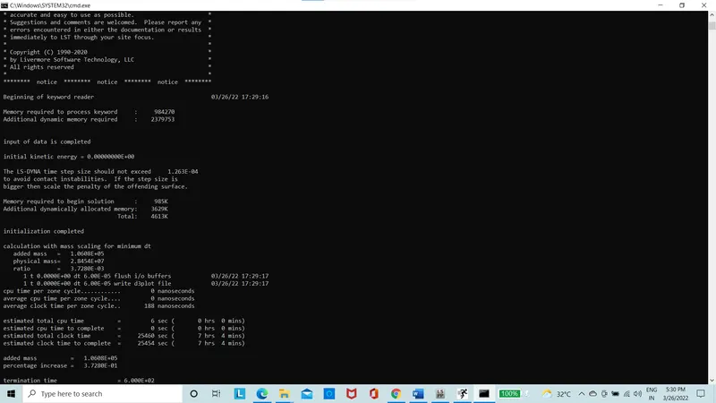
Figure 10: Model with DT2MS as -7.5E-5
The model is now added with mass by giving the value of TSSFAC=0.8 and DT2MS=-8.5E-5
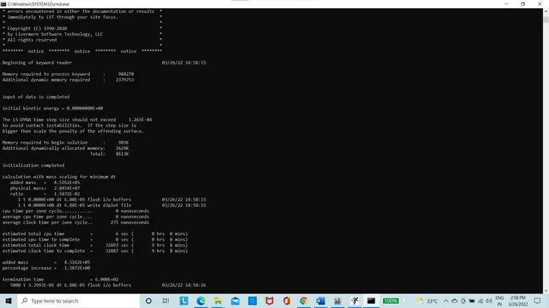
Figure 11: Model with DT2MS as -8.5E-5
The model is now added with mass by giving the value of TSSFAC=0.8 and DT2MS=-9.5E-5
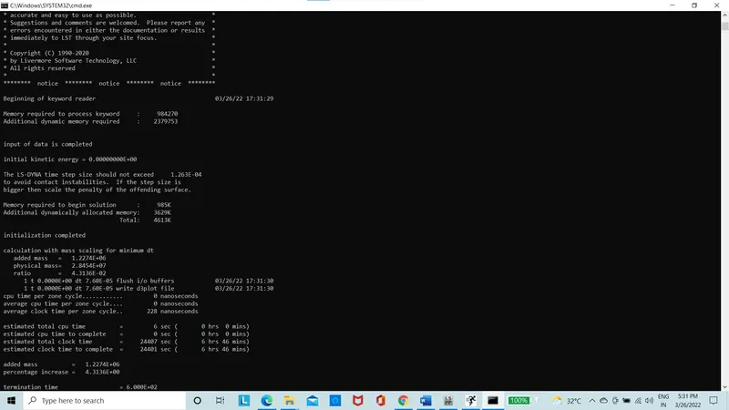
Figure 12: Model with DT2MS as -9.5E-5
The model is now added with mass by giving the value of TSSFAC=0.9 and DT2MS=-1.03E-4
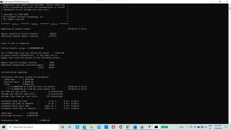
Figure 13: Model with DT2MS as -1.03E-4
The value of DT2MS is not further increased as the value of percentage increased will increase more than the hard limit of 8%, therefore will stop the iteration till DT2MS is -1.03E-4.
The values of the TSSFAC=0.9 and TSSFAC=0.8 Verses timestep is plotted
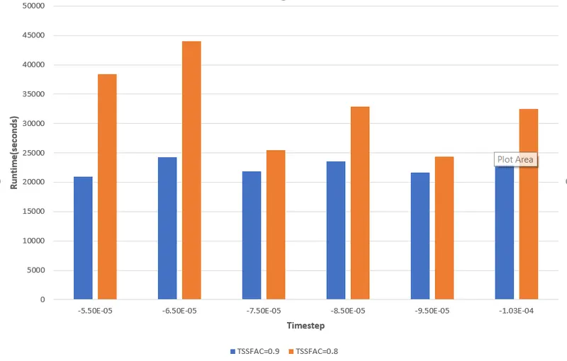
Figure 14: Chart Runtime verses Timestep
Finally, Implicit Analysis is run to find out how the simulation behaves and the difference in the run time compared to explicit analysis, therefore we need to add the implicit general, implicit auto, implicit solver, implicit solve in the control option.
In the implicit general, IMFLAG is set to 1 for implicit analysis, in implicit auto, IAUTO is set to 1, Implicit solution is taken as default, implicit solver is also taken as default and the simulation is run.
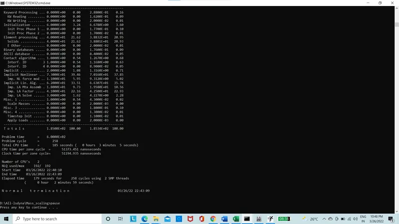
Figure 15: Implicit Command File
Here, in implicit analysis the run time is very low compared to the explicit analysis since, the timestep is more defined in implicit than in explicit analysis.
Conclusion:
The time step is increased using the mass scaling for the explicit analysis by adding artificial mass to the element required and the run time is reduced subsequently. When implicit analysis is used there is very large gap in run time compared with explicit analysis. The implicit analysis taken few minutes, whereas the explicit takes hours to solve the simulation.