#11 Braking

1.For a defined driving cycle, calculate the energy required for braking.

clear all
close all
clc
load Myowndrivecycle.txt                  % to load my drive cycle
time = Myowndrivecycle (:,1);
Speed = Myowndrivecycle (:,2);
figure(1)
plot (time,Speed)                         % to plot the given drive cycle
title ('DriveCycle')                      % title for the graph
hold on
xlabel ('time (s)')                       % labelling X-Axis
ylabel ('Speed (m/s)')                    % labelling Y-Axis
Kerb_Weight = 1000 ;                      % Vehicle Weight in Kg
brake_Energy = (0.5.*Kerb_Weight.*Speed.^2)./1000; % formula for brake energy E=1/2*m*v^2
figure(2)
plot (time,brake_Energy)                  % to plot calculated brake energy
title ('Brake energy Vs Time')
hold on 
xlabel ('time (s)')                       % labelling X-Axis
ylabel ('Brake Energy (KJ)')              % labelling Y-Axis

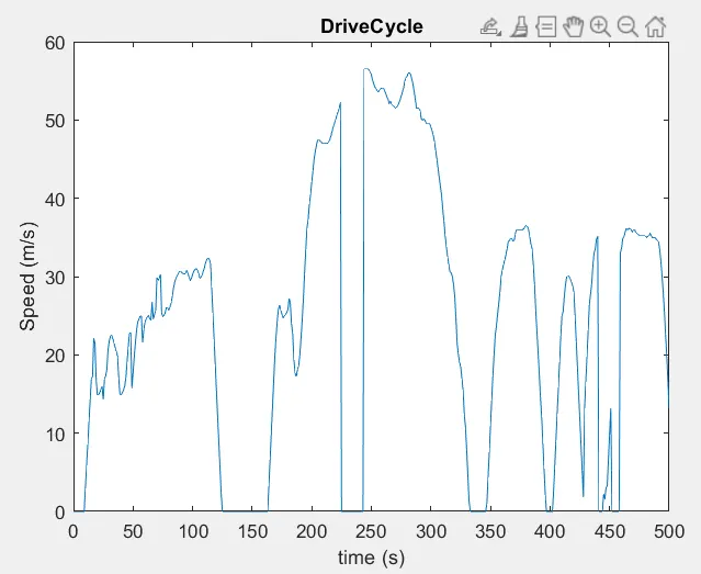
First i have created a drivecycle data in txt format and load the file in my script file.

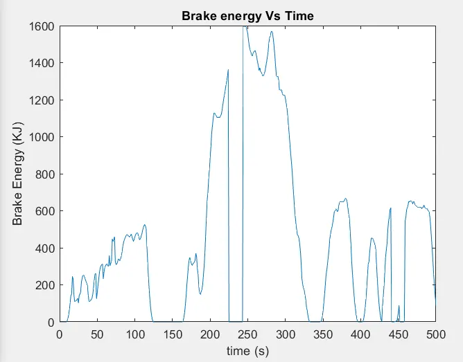
plot the given drive cycle and calculate the enegry required for braking using the formula E=1/2*m*v^2.

again plot the calculated braking energy.

The obtained plots are

2.Why electric motor can’t develop braking torque at high speed similar to starting? How electric and mechanical brakes are coordinated?

Co-ordination of electric and mechanical Brakes:

There are three different types of braking control strategies

1. Braking with optimal braking feel
2. Series braking with optimal energy
3. parallel braking

The typical braking control strategy include the best brake feeling, the best energy recovery and parallel
type braking control strategy , in which the former two that firstly consider the regenerative braking,
and then to mechanical braking belong to serial braking control strategy. In contrast, the mechanical and
regenerative braking are parallel and simultaneously produce braking force in the condition of the
parallel braking.

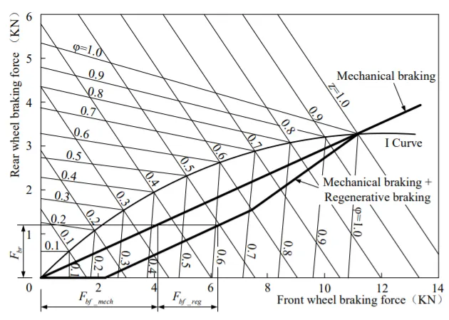
The mechanical braking of the parallel braking system can distribute the braking force of the front
and rear wheels in a fixed proportion and the regenerative braking supplement the braking force
insufficient on supplementary driving wheel, which forms the distribution curve of braking force
required by the driver.
The mechanical friction braking force applied on the front and rear axle is in direct proportion with
the hydraulic pressure in the brake master cylinder. Regenerative braking force is a function of the
hydraulic pressure in the main cylinder. Regenerative braking force is a function of the hydraulic
pressure in the brake master cylinder, which is also a function of the deceleration speed of vehicles
braking.
The basic strategy of the parallel braking control strategy:
(1) When z is larger
When the braking strength of vehicles is larger(such as z =0.9), the braking energy is less due to the
shorter braking time, and the driving motor does not produce regenerative braking force to guarantee
the braking safety.
(2) When z is smaller
During the process of braking, regenerative braking is effective when z is less than 0.9.
(3) When z is very small
During the process of braking, when the z is less than a certain value, such as 0.1, it will just
require the regenerative braking.

The series-parallel regenerative braking control strategy of hybrid electric vehicle is designed
according to the basic idea of parallel braking control strategy as well the characteristics of regenerative
braking system of hybrid electric vehicle and the working characteristics of key components of
regenerative braking system such as driving motor and power battery.
Set the z as the reference, and distribute the mechanical braking force and regenerative braking
force to ensure the braking efficiency and recover as much braking energy as possible.

3.Make a MATLAB program which plots contour of given motor speed, torque and efficiency values. Attach the code as a .m file attach a screenshot of all the plots.

clear all
close all
clc
W = linspace(0,1250,250);
T = linspace(0,100,250);
%Motor constants
Kc = 0.2; % for copper loss
Ki = 0.008; %for Iron lOss
Kw = 0.00001; % for windage loss
cont = 20; %for constant motor loss
%making mesh 
[X,Y] = meshgrid(W,T);
Outputpower = (X .* Y); %Torque*speed = power
B = (Y .^ 2)*Kc; % Copper loss
C = (X .^ 3)*Kc; %winding loss
D = X .* Ki; % Iron loss
Inputpower = Outputpower + B + C + D + cont;
Z = Outputpower ./ Inputpower;
% Set the efficiencies for which the controll will be plotted
V = [0.70,0.80,0.85,0.90,0.91,0.20,0.925,0.93];
figure 
box off
grid off
contourf (X,Y,Z,V)
colorbar
xlabel ('Speed (rad/sec)')
ylabel ('Torque (N.m)')
zlabel ('Efficiency')
title ('Torque-Speed curve for the induction motor')

figure 
surf (X,Y,Z); 
colorbar;
xlabel ('Speed (rad/sec)')
ylabel ('Torque (N.m)')
zlabel ('Efficiency')
title ('Efficiency curve for the Induction Motor')

xlabel ('Speed (rad/sec)')
ylabel ('Torque (N.m)')
zlabel ('Efficiency')

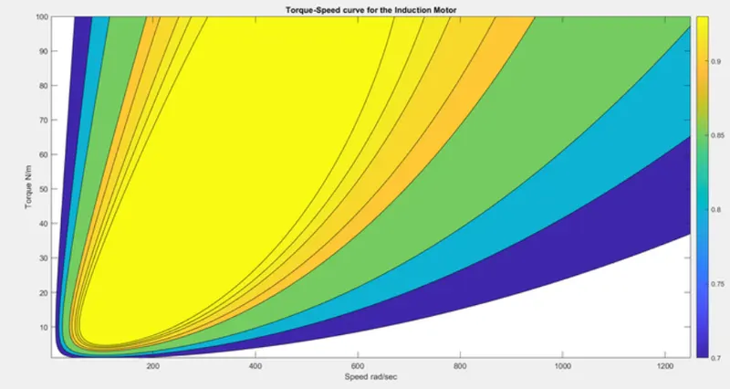
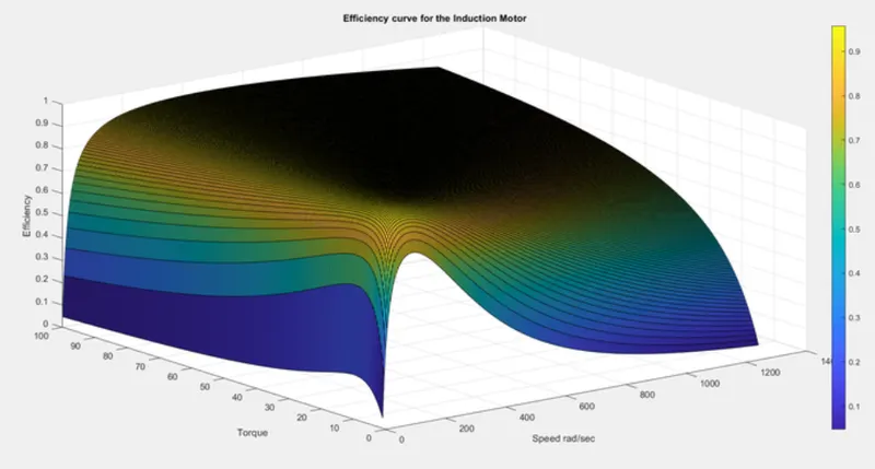
here i have defined arrays for speed and torque of the motor. then they are plot in a 2D coordinate, using the command meshgrid. followed by the loss constants for calculating the losses occuring in the motor. These losses are used in calculating input and output power, followed by the efficiency of the motor. The array V is defined with the values of efficiency for which we want to plot. Finally the contour plot is defined. In the contour command, the variable ''Z'' is defined as the function of X and Y followed by V for plotting the efficiency contour.

Motor Losses:

• Copper loss = Kc
• Iron loss = Ki
• Windage loss = Kw
• Conduction loss

The output plot obtained are