Simulation of steady and unsteady flow over a cylinder

Aim:

To simulate the flow over a cylinder and explain the phenomenon of Karman vortex street.

Problem statement:

PART-I

1. Simulate the flow with the steady and unsteady case and calculate the Strouhal Number for Re=100.

PART-II

1. Calculate the coefficient of drag and lift over a cylinder by setting the Reynolds number to 10, 100, 1000, 10000, and 100000 using the steady-state solver
2. Discuss the effect of Reynolds number on the coefficient of drag (Cd).

Theory:

1. Karman vortex sheet:

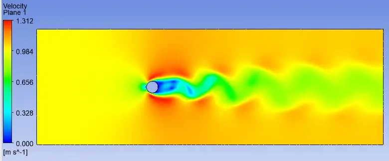
The Karman vortex street is a repeating pattern of swirling vortices, caused by a process known as vortex shedding, which is responsible for the unsteady separation of flow of a fluid around blunt bodies.

2. Reynolds number:

The Reynolds number is the ratio of inertial forces to viscous forces within a fluid that is subjected to relative internal movement due to different fluid velocities.

`Re=(rho.v.D)/mu`

Where `rho=`Density of the fluid

v= Velocity of the flow of the fluid

D= Diameter of the cylinder

`mu=` Dynamic viscosity of the fluid

3. Strouhal Number:

The Strouhal number is a dimensionless number describing oscillating flow mechanisms.

`St=(f*L)/v`

where f= The frequency of vortex shedding

L= Characteristic length

v= Flow velocity

4. coefficient of drag(Cd):

The drag coefficient (Cd) is a dimensionless quantity that is used to quantify the drag/resistance of an object in a fluid environment.

`Cd=(2*D)/(rho*v^2*A)`

Where D= Drag force

`rho=`Density of the fluid

v= Flow velocity

A= Reference area

5. coefficient of lift(Cl):

The lift coefficient (C_L) is a dimensionless quantity that relates the lift generated by a lifting body to the fluid density around the body, the fluid velocity, and an associated reference area.

`Cl=(2*L)/(rho*v^2*A)`

Where L= Lift force

Geometry:

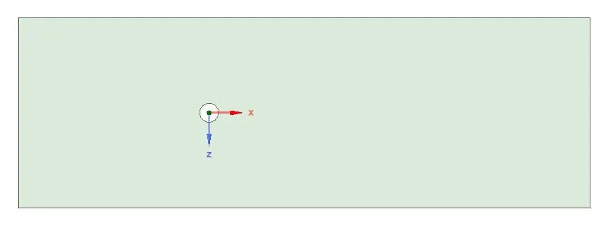
Since we are performing a 2D analysis of the flow of the fluid over the cylinder, the length of the cylinder is not given importance, only its cross-section is taken into consideration. The diameter of the cylinder is 2m. This cylinder cross-section is drawn at the origin of the x-z plane. To simulate flow over the cylinder, a control volume/area is modeled, this can also be called as the virtual wind tunnel. The dimensions of the control area are 20x60m. The distance from the center of the cylinder to the inlet is 20m, and the outlet is 40m. The distance between the center of the cylinder and the top and bottom wall is 10m each.

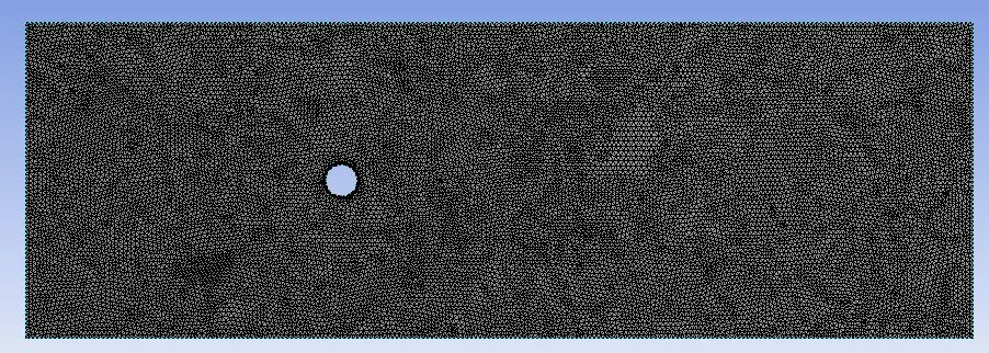
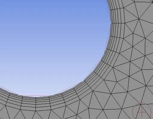
Now that we have modeled the 2D geometry of the cylinder and the virtual wind tunnel, meshing needs to be done. The element size is taken as 0.25m, with the element geometry as triangles. To get accurate results near the wall of the cylinder, 6 inflation layers are introduced, with the first layer having a size of 0.244m and the subsequent elements having a growth rate of 1.2. This value is calculated using an online calculator 'Pointwise'. The wall is sized to have 36 elements to get smooth edges. Once this mesh is generated there will be a total of 40404 mesh elements.

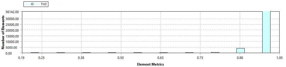
Since the majority of the mesh elements have mesh quality above 80%, and there are no mesh elements with the mesh quality less than 20%, the generated mesh is said to be of good quality, and simulations can be run using this mesh.

Part I:

Boundary conditions:

1. Dynamic viscosity= 0.02Ns/m^2
2. Flow velocity= 1m/s
3. Densty of the fluid= 1kg/m^3
4. The diameter of the cylinder= 2m

Steady-state analysis:

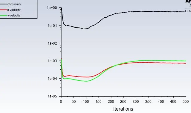
The solution was run for 500 iterations, and from the trend of the residuals plot, we can say that the solution is converged after 300 iterations.

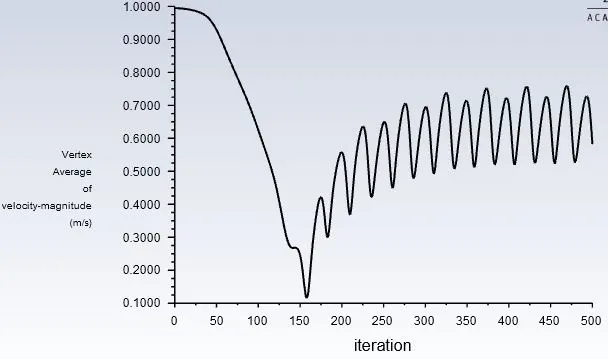
To visualize the formation of the Karman vortex sheet behind the cylinder, a point is created 10m behind the cylinder, and the vortex average of velocity is plotted. From the trend of this plot, we can see that initially, the vortex velocity keeps dropping up to around 150 iterations, after this, there is an increase in this magnitude, and further this there will be a formation of vertex sheet. Once the solution is converged, the oscillations of the velocity vortex average stabilize. The vortex velocity magnitude, once the solution is stabilized, varies constantly from approximately 0.55-0.75m/s. Since the steady-state analysis is not time accurate, the Strouhal number cannot be calculated since it contains the term vortex frequency which is a function of time. Hence, to calculate the Strouhal number, the transient-state analysis must be used. Nevertheless, the steady-state analysis is used to simulate the solution once it has reached the steady-state condition.

Transient state analysis:

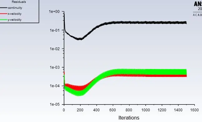
The solution was run for 300 time-steps, with each time-step performing 5 iterations. From the trend of the residuals plot, we can say that the solution is converged after 500 iterations.

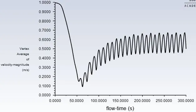
To visualize the formation of the Karman vortex sheet behind the cylinder, a point is created 10m behind the cylinder, and the vortex average of velocity is plotted. From the trend of this plot, we can see that initially, the vortex velocity keeps dropping up to around 50 iterations, after this, there is an increase in this magnitude, and further this there will be a formation of vertex sheet. Once the solution is converged, the oscillations of the velocity vortex average stabilize. The vortex velocity magnitude, once the solution is stabilized, varies constantly from approximately 0.45 to 0.7m/s.

The Strouhal number can be calculated using the Strouhal number formula and is given by St=`(f.L)/v=((10/100)*2)/1=0.2`

Part II

Boundary conditions:

1. Dynamic viscosity= 0.02Ns/m^2
2. Densty of the fluid= 1kg/m^3
3. The diameter of the cylinder= 2m
4. To obtain Reynolds number of 10, 100, 1000, 10000, and 100000, the flow velocity at the inlet must be given as 0.1, 1, 10, 100, and 1000m/s respectively.
5. The solver used: Steady-state

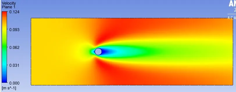
1. Reynolds number 10:

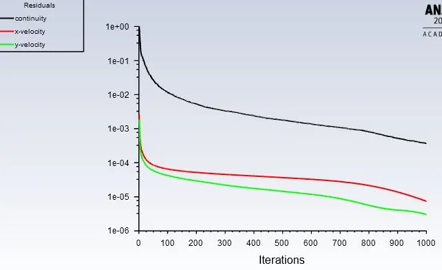
The solution was run for 1000 iterations, and we can say that the solution has converged since the residuals plot has dipped below 1e-03.

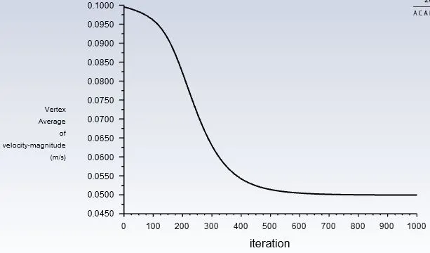
A point is created 10m behind the cylinder, and the vortex average of velocity is plotted. From the trend of this plot, we can see that initially, the vortex velocity keeps dropping up to around 450 iterations, after this, the magnitude of vortex velocity remains fairly constant at around 0.05m/s. There is no formation of Karman vortex sheet for flow over a circular cylinder with Reynolds number 10

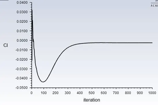
From the coefficient of lift plot, since there is no vortex formation for flow with Reynolds number 10, the coefficient of lift solution converges after approximately 400 iterations. The corresponding value is around zero.

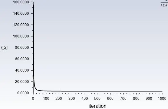
the coefficient of drag solution converges after approximately 50 iterations. The corresponding value is around 5.

2. Reynolds number 100

The solution was run for 500 iterations, and from the trend of the residuals plot, we can say that the solution is converged after 300 iterations.

To visualize the formation of the Karman vortex sheet behind the cylinder, a point is created 10m behind the cylinder, and the vortex average of velocity is plotted. From the trend of this plot, we can see that initially, the vortex velocity keeps dropping up to around 150 iterations, after this, there is an increase in this magnitude, and further this there will be a formation of vertex sheet. Once the solution is converged, the oscillations of the velocity vortex average stabilize. The vortex velocity magnitude, once the solution is stabilized, varies constantly from approximately 0.55-0.75m/s.

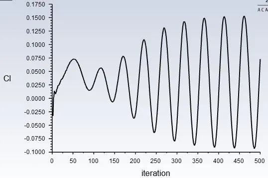
Since there is a formation of the Karman vortex sheet for fluid with Reynolds number 100, the value of the coefficient of lift varies and does not have a fixed value. These oscillations stabilize after approximately 300 iterations. One these oscillations are stabilized, the coefficient of lift varies from approximately from -0.0875 to 0.15

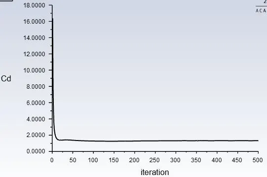
The coefficient of drag solution converges after approximately 25 iterations. The corresponding value is around 1.75.

3. Reynolds number 1000

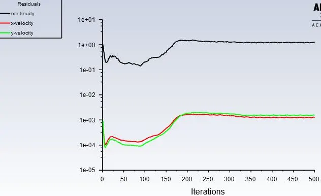
The solution was run for 500 iterations, and from the trend of the residuals plot, we can say that the solution is converged after 200 iterations.

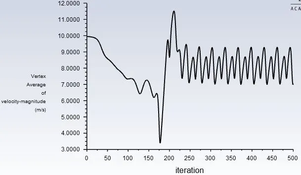
To visualize the formation of the Karman vortex sheet behind the cylinder, a point is created 10m behind the cylinder, and the vortex average of velocity is plotted. From the trend of this plot, we can see that initially, the vortex velocity keeps dropping up to around 150 iterations, after this, there is an increase in this magnitude, and further this there will be a formation of vertex sheet. Once the solution is converged, the oscillations of the velocity vortex average stabilize. The vortex velocity magnitude, once the solution is stabilized, varies constantly from approximately 7 to 9m/s.

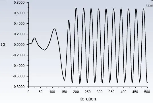
Since there is a formation of the Karman vortex sheet for fluid with Reynolds number 1000, the value of the coefficient of lift varies continuously and does not have a fixed value. These oscillations stabilize after approximately 200 iterations. One these oscillations are stabilized, the coefficient of lift varies from approximately from -0.7 to 0.7.

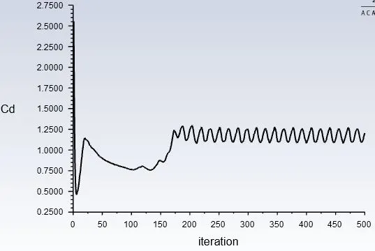
the coefficient of drag solution converges after approximately 200 iterations. The corresponding value is around 1 to 1.25.

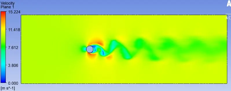
4. Reynolds number 10000

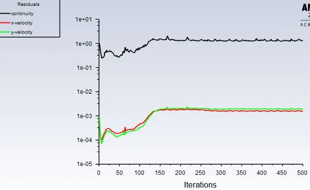
The solution was run for 500 iterations, and from the trend of the residuals plot, we can say that the solution is converged after 150 iterations.

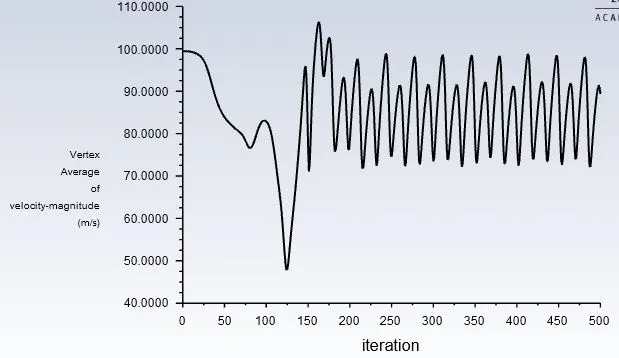
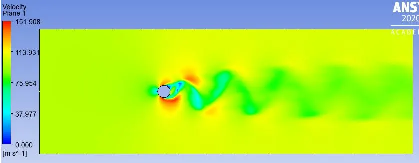
To visualize the formation of the Karman vortex sheet behind the cylinder, a point is created 10m behind the cylinder, and the vortex average of velocity is plotted. From the trend of this plot, we can see that initially, the vortex velocity keeps dropping up to around 125 iterations, after this, there is an increase in this magnitude, and further this there will be a formation of vertex sheet. Once the solution is converged, the oscillations of the velocity vortex average stabilize. The vortex velocity magnitude, once the solution is stabilized, varies constantly from approximately 75 to 100m/s.

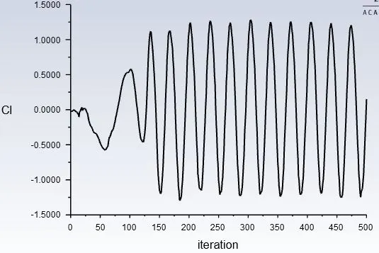
Since there is a formation of the Karman vortex sheet for fluid with Reynolds number 10000, the value of the coefficient of lift varies and does not have a fixed value. These oscillations stabilize after approximately 150 iterations. One these oscillations are stabilized, the coefficient of lift varies from approximately from -1.25 to 1.25.

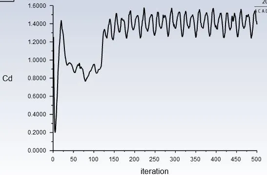
the coefficient of drag solution converges after approximately 200 iterations. The corresponding value oscillates from 1.3 to 1.6.

5. Reynolds number 100000

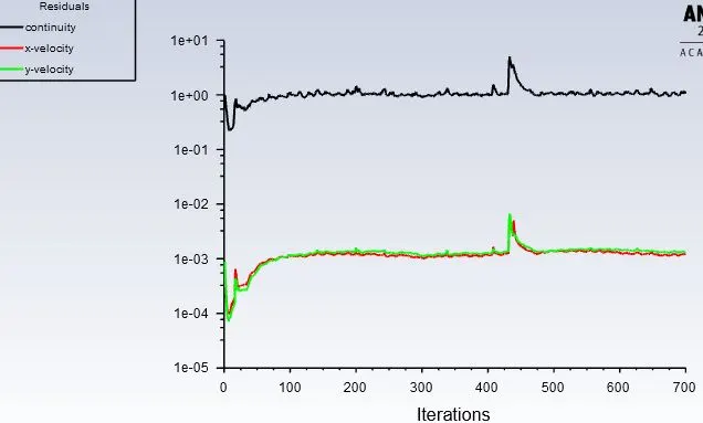
The solution was run for 700 iterations, and from the trend of the residuals plot, we can say that the solution is converged after 500 iterations.

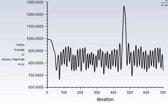
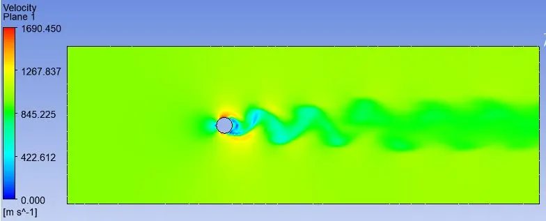
To visualize the formation of the Karman vortex sheet behind the cylinder, a point is created 10m behind the cylinder, and the vortex average of velocity is plotted. From the trend of this plot, we can see that initially, the vortex velocity keeps dropping up to around 150 iterations, after this, there is an increase in this magnitude, and further this there will be a formation of vertex sheet. Once the solution is converged, the oscillations of the velocity vortex average stabilize. The vortex velocity magnitude, once the solution is stabilized, varies constantly from approximately 700 to 900m/s.

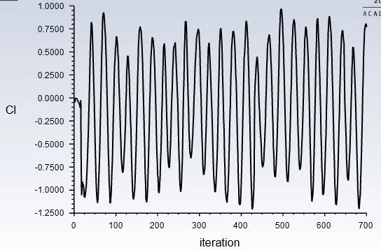
Since there is a formation of the Karman vortex sheet for fluid with Reynolds number 100000, the coefficient of lift keeps oscillating from approximately -1 to 1.

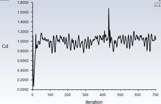
The coefficient of drag value keeps oscillating from approximately 0.8 to 1.2 once the solution is converged.

Results and conclusions:

1. For a particular Reynolds number, it is easier to calculate the Stroudal number of a vortex flow if it is solved using transient-state analysis than the steady-state analysis both analytically and through software. This is mainly because the steady-state analysis does not estimate time accurate results, it rather predicts the solution once it has reached the steady-state. On the other hand, the transient-state analysis gives time accurate results, hence the vortex shedding frequency can be calculated easily, and subsequently, the Stroudal number calculated.
2. For smaller Reynolds numbers, the flow is laminar, hence, the oscillations produced by the vortex average of velocity remain fairly uniform. For flow with higher Reynolds number, these oscillations tend to be more and more un-organized
3. For flow with Reynolds number of 10, there was no formation of the vortex sheet. This phenomenon usually occurs when the fluid flow has a Reynolds number of 40 and beyond. In the laminar regime, ie, for a flow with Reynolds number below 2100, the vortex oscillations remain fairly uniform once it has reached the steady-state condition. For flow in the turbulent regime, these oscillations become more unstable with the increase in the Reynolds number.
4. Even the coefficient of lift keeps oscillating about a point for flows with Reynolds number greater than 40, ie, for flows where the Karman vortex shedding is observed. In the case of flow with Reynolds number of 10, the coefficient of lift is almost zero.
5. In the laminar regime, the coefficient of drag increases with the increase in the Reynolds number of the flowing fluid.
6. During the meshing of the model, enough inflation layers must be provided, and the mesh sizing must be as small as possible so as to retain the original shape of the geometry. Doing this will increase the accuracy of the solution obtained.