Simulation of flow over a backward facing step
Aim:
To simulate the turbulent flow of air in a backward-facing step for different base grid sizes and draw suitable conclusions
Theory:
The separated flow generated as fluid passes over a backward-facing step is of interest for a variety of reasons. First, separated flows produced by an abrupt change in the geometry are of great importance in many engineering applications. Also, the backward-facing step is an extreme example of separated flows that occur in aerodynamic devices such as high-lift airfoils at large angles of attack. In these flows, separation may be created by a strong adverse pressure gradient rather than a geometric perturbation, but the flow topology is similar. Secondly, from a fundamental perspective, there is a strong interest in understanding instability and transition to turbulence in non-parallel open flows. Hence, transition mechanisms in parallel flows such as plane channels and pipes have received substantial attention.
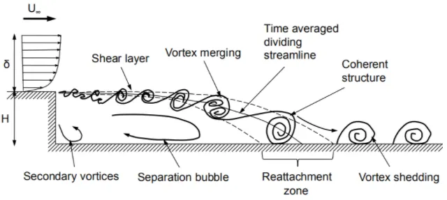
The general characteristics of the backward-facing step flow begin with an upstream boundary layer separating at the step edge due to the adverse pressure gradient that develops into a thin shear layer. The size of the shear layer increases downstream. It consists of many vortices and further vortices start merging together to form larger vortices. The shear layer becomes the shear zone when the size of the shear layer increases due to vortices, coherent structures. Finally, the separated flow attaches with the bottom of the BFS when a favorable pressure gradient is obtained. The point of reattachment is known as the reattachment point. The distance between the wall of the step and the reattachment point is known as the reattachment length. The location of the reattachment point is unsteady due to the inherent oscillatory motion of the shear layer. Hence, the reattachment zone is formed in which the reattachment point can present. The turbulent structures in the shear layer entrain irrotational fluid outside the shear zone. This creates low-velocity circulation between the step wall and the shear zone. This leads to the formation of the recirculation zone. The recirculation zone is mainly comprised of a primary vortex in the center and a secondary vortex adjacent to the corner of the step.
Geometry:
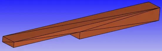
The length of the backward-facing channel is 0.272m, and the dimensions of the inlet and outlet are 0.01m and 0.02m respectively. Since we are performing a 2D simulation on the given backward-facing step, the length of the channel in the z-direction is not important. The faces of the geometry are given different names(inlet, outlet, front_2d, back_2d, and top_bottom) so that the boundary conditions can be provided easily.
Case setup:
1. Mesh sizes
Mesh element sizes in x, y, and z-directions:
case1: 2e-3m
case2: 1.5e-3m
case3: 1e-3m
2. Type of simulation: Steady-state simulation with zero reactions and only air(77% N2, 23% O2) as the medium of flow.
3. Steady-state monitor properties:
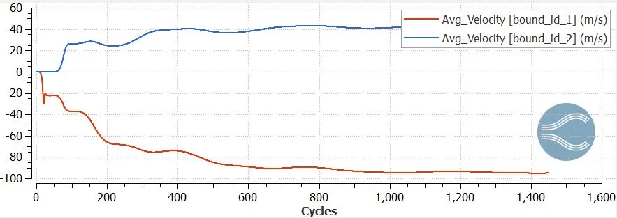
a) Average velocity at the outlet
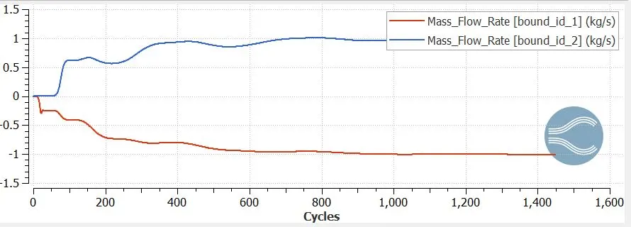
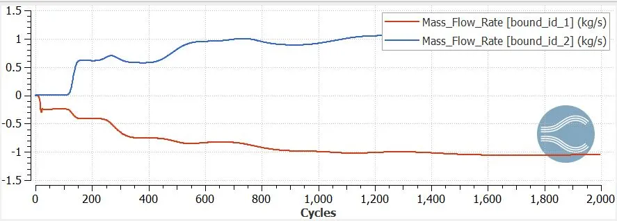
b) Average mass flow rate at the outlet
4. Boundaries:
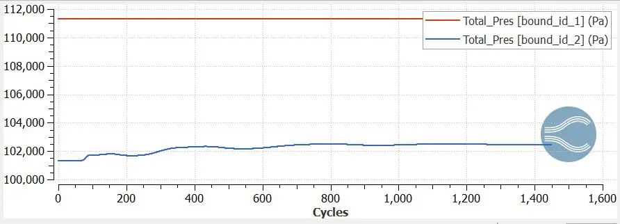
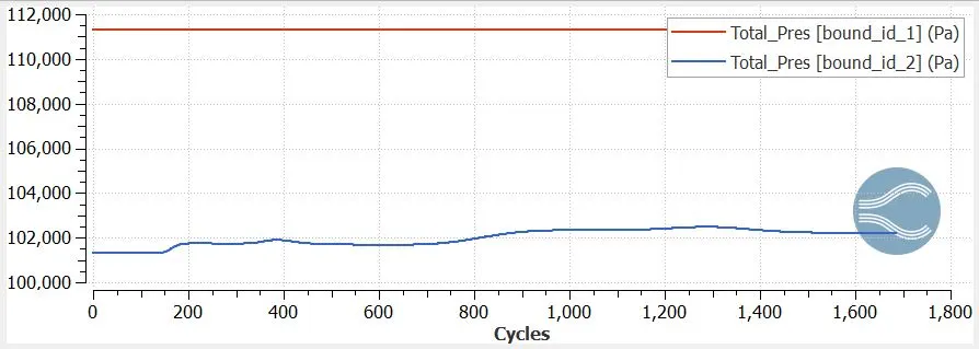
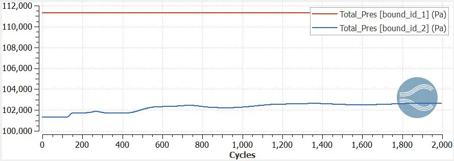
Inlet: Inflow boundary condition with pressure inlet (111325Pa).
Outlet: Outflow boundary condition with pressure outlet (101325Pa).
Top and Bottom: Stationary, no-slip wall.
Front and Back: 2D faces.
Pressure difference between the inlet and outlet= 10000Pa
5. Solver properties:
Details: 2 minimum iterations and 20 max iterations per cycle. Tolerance = 0.001
Minimum Cycles = 0
Maximum Cycles = 15000
Minimum time step = 1e-9 sec
Maximum time step = 1 sec
Maximum convection CFL limit(final stage)= 0.5
6.Turbulence model:
RNG K-epsilon turbulence model
Results:
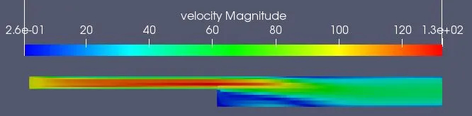
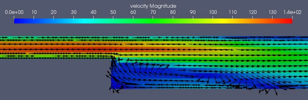
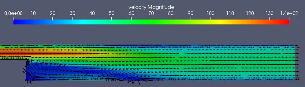
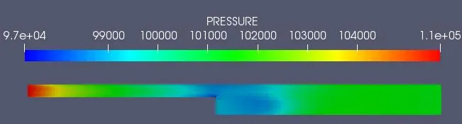
Case1: mesh grid size= 2e-3m
mesh:
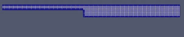
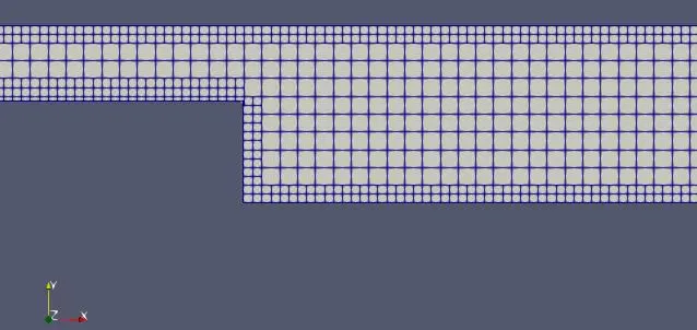
One fixed embedding layer was provided near the wall of scale 1. The total number of mesh elements is 1943
Velocity contours:
Pressure contours:
Line plots:
Average velocity:
Total pressure:
Mass flow rate:
Cell count:
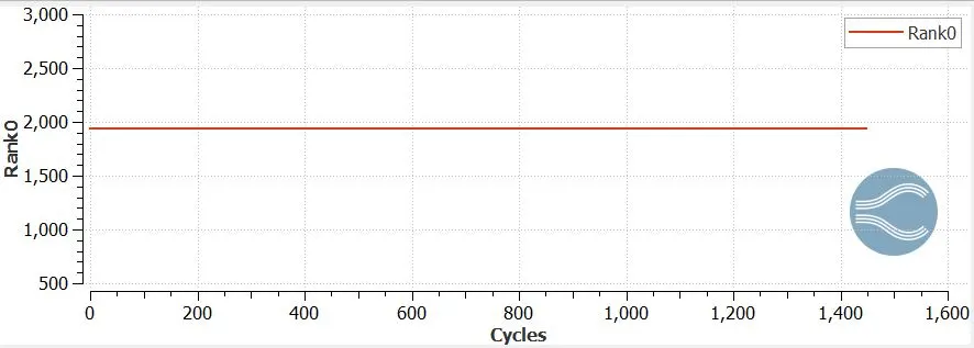
Total number of cells generated and solved by the processor= 1943
Case2: Mesh grid size= 1.5e-3m
Mesh:
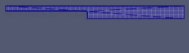
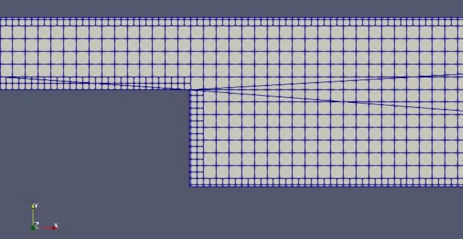
One fixed embedding layer was provided near the wall of scale 1. The total number of mesh elements is 2994
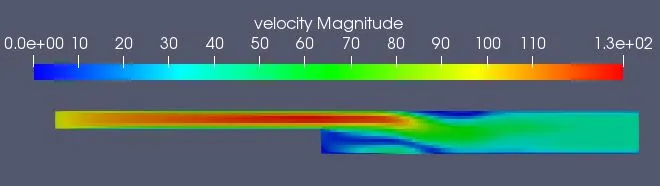
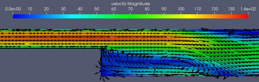
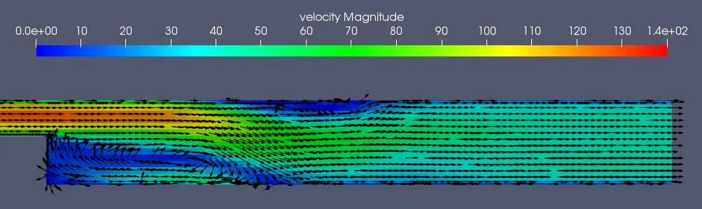
Velocity contours:
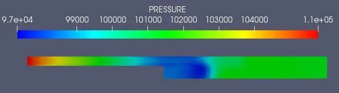
Pressure contours:
Line plots:
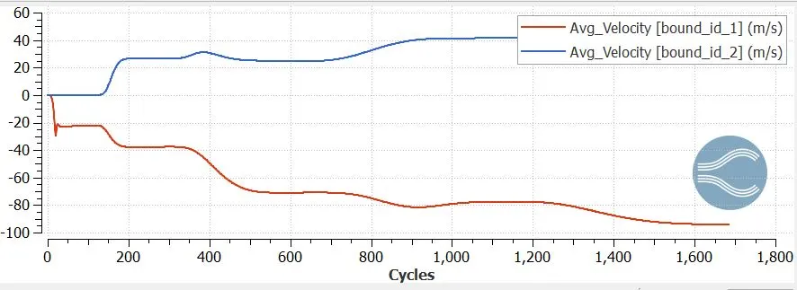
Average velocity:
Total pressure:
Mass flow rate:
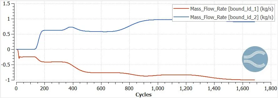
Cell count:
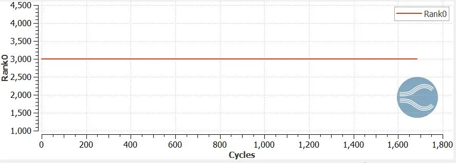
Total number of cells generated and solved by the processor= 2994
Case3: Mesh grid size= 1e-3m
Mesh:
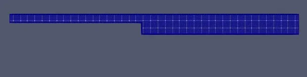
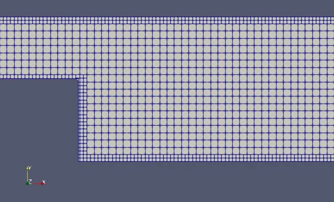
One fixed embedding layer was provided near the wall of scale 1. The total number of mesh elements is 5516
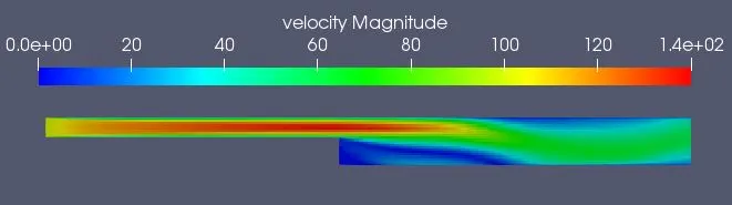
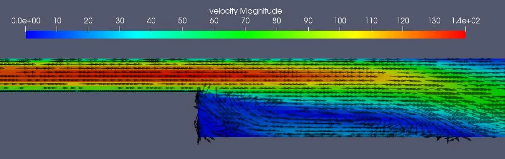
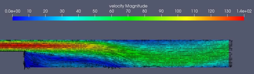
Velocity contours:
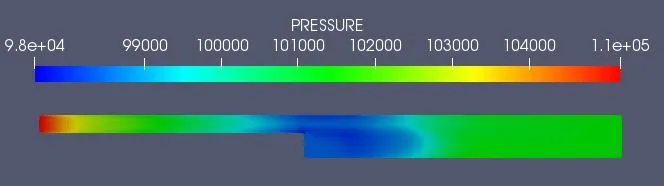
Pressure contours:
Line plots:
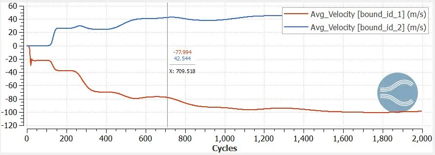
Average velocity:
Total pressure:
Mass flow rate:
Cell count:
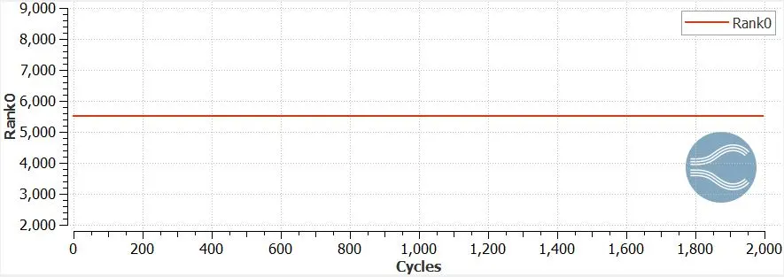
Total number of cells generated and solved by the processor= 5516
Conclusions:
The flow simulation of air was performed on the backward-facing step for 3 different mesh sizes and the following conclusions can be drawn:
- The air flows from the inlet to the outlet. The velocity of air is higher at the inlet than at the outlet. This is because of the backward-facing step, which changes the geometry of the fluid domain.
- Due to the backward-facing step, there is a pressure drop near the step, this causes some fluid particles to flow in the reverse direction, which creates vortices. This can be clearly seen in the vector plot.
- With the increase in the number of grid elements, the solution obtained becomes more and more accurate. The flow properties are captured more accurately if the mesh is more refined. This is the reason for the introduction of embedded layers which improves the accuracy of the solution near the walls. In general, the smaller the element size, the more accurate is the solution obtained.
- With the increase in the number of cells, the solution becomes more accurate but the computation time increases considerably. Hence, the problem must be studied thoroughly before performing the simulation and it must be decided how much are we willing to compromise the accuracy of the solution to save resources.