Simulation of flow over a NACA 2412 airfoil

Aim:

1. To compare the results obtained at a particular angle of attack using different turbulence models with experimental data and choose the better turbulence model to solve the problem for the remaining angle of attacks.
2. To simulate the flow over NACA 2412 airfoil and find the coefficient of lift and drag at different angles of attack.

Theory:

An airfoil is the cross-sectional shape of a wing, blade (of a propeller, rotor, or turbine), or sail (as seen in cross-section). An airfoil-shaped body moving through a fluid produces an aerodynamic force. The component of this force perpendicular to the direction of motion is called lift. The component parallel to the direction of motion is called drag. Subsonic flight airfoils have a characteristic shape with a rounded leading edge, followed by a sharp trailing edge, often with a symmetric curvature of upper and lower surfaces. Foils of similar function designed with water as the working fluid are called hydrofoil. Airfoil's lift coefficient can be increased by using flaps at the end of the airfoil without much increase in drag.

The lift on an airfoil is primarily the result of its angle of attack. Most foil shapes require a positive angle of attack to generate lift, but cambered airfoils can generate lift at zero angle of attack. This "turning" of the air in the vicinity of the airfoil creates curved streamlines, resulting in lower pressure on one side and higher pressure on the other. This pressure difference is accompanied by a velocity difference, via Bernoulli's principle, so the resulting flowfield about the airfoil has a higher average velocity on the upper surface than on the lower surface. In some situations (e.g. inviscid potential flow) the lift force can be related directly to the average top/bottom velocity difference without computing the pressure by using the concept of circulation and the Kutta–Joukowski theorem.

Airfoil design is a major facet of aerodynamics. Various airfoils serve different flight regimes. Asymmetric airfoils can generate lift at zero angle of attack, while an symmetric airfoil may better suit frequent inverted flight as in an aerobatic airplane. In the region of the ailerons and near a wingtip a symmetric airfoil can be used to increase the range of angles of attack to avoid spin–stall. Thus a large range of angles can be used without boundary layer separation. Subsonic airfoils have a round leading edge, which is naturally insensitive to the angle of attack. The cross-section is not strictly circular, however: the radius of curvature is increased before the wing achieves maximum thickness to minimize the chance of boundary layer separation. This elongates the wing and moves the point of maximum thickness back from the leading edge.

Supersonic airfoils are much more angular in shape and can have a very sharp leading edge, which is very sensitive to the angle of attack. A supercritical airfoil has its maximum thickness close to the leading edge to have a lot of length to slow shock subsonic speeds. Generally, such transonic airfoils and also supersonic airfoils that have a low camber to reduce drag divergence. Modern aircraft wings may have different airfoil sections along the wingspan, each one optimized for the conditions in each section of the wing. Movable high-lift devices, flaps and slats, are fitted to airfoils on almost every aircraft. A trailing edge flap acts similarly to an aileron; however, it, as opposed to an aileron, can be retracted partially into the wing if not used.

Airfoil nomenclature:

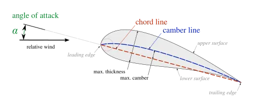
The geometry of the airfoil is described with a variety of terms :

• The leading edge is the point at the front of the airfoil that has the maximum curvature (minimum radius).
• The trailing edge is defined similarly as the point of maximum curvature at the rear of the airfoil.
• The chord line is the straight line connecting leading and trailing edges. The chord length, is the length of the chord line. That is the reference dimension of the airfoil section.

The shape of the airfoil is defined using the following geometrical parameters:

• The mean camber line is the locus of points midway between the upper and lower surfaces. Its shape depends on the thickness distribution along the chord
• The thickness of an airfoil varies along the chord. It may be measured in either of two ways:
  • Thickness measured perpendicular to the camber line.
  • Thickness measured perpendicular to the chord line.

Common terms used to describe the airfoil's behaviour when it is moving through a fluid are:

• The aerodynamic center is the chord-wise length about which the pitching moment is independent of the lift coefficient and the angle of attack.
• The center of pressure is the chord-wise location about which the pitching moment is zero.

Main types of NACA airfoil:

The NACA four-digit wing sections define the profile by:

1. First digit describing maximum camber as a percentage of the chord.
2. The second digit describing the distance of maximum camber from the airfoil leading edge in tenths of the chord.
3. Last two digits describing the maximum thickness of the airfoil as a percent of the chord.

The NACA five-digit series describes more complex airfoil shapes. Its format is LPSTT, where:

• L: a single digit representing the theoretical optimal lift coefficient at the ideal angle of attack C_LI = 0.15 L
• P: a single digit for the x coordinate of the point of maximum camber.
• S: a single-digit indicating whether the camber is simple (S = 0) or reflex (S = 1),
• TT: the maximum thickness in percent of the chord, as in a four-digit NACA airfoil code.

Problem-solving methodology:

Part1:

To simulate the flow over NACA 2412 airfoil at a zero-degree angle of attack using RNG K-epsilon and K-omega SST turbulence model at the same initial conditions, boundary conditions, and case setup and compare the results obtained with experimental data. The part 2 proble is solved using the turbulence model which give more accurate results.

Part2:

The flow is simulated on the NACA 2412 airfoil at 1, 5, 10, and 15-degree angles of attack using the turbulence model chosen in part1, and the coefficient of drag vs angle of attack and coefficient of lift vs angle of attack is plotted and relevant conclusions are drawn.

Geometry:

The NACA 2412 coordinate points for chord length 0.1m were imported from airfoiltools.com into CATIA (a CAD software), and the required airfoil was generated by joining these coordinate points using the spline tool. This airfoil geometry is enclosed by a box (virtual wind tunnel) and is saved in STL format. The different angles of attack can be obtained by using the rotate tool. Once the geometry is saved in STL format, it can be imported into Converge CFD and simulations performed.

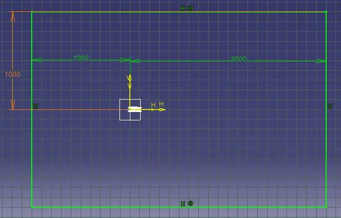
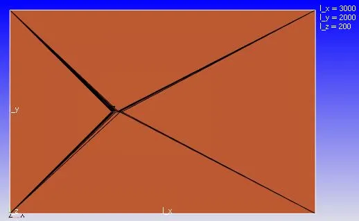
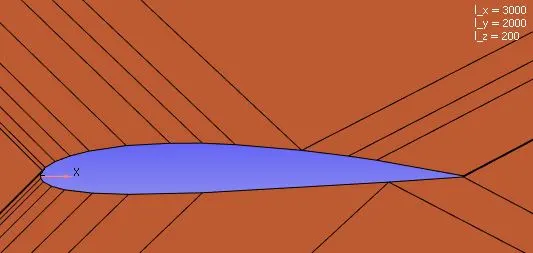
In CATIA, all the dimensions are provided in millimeters, when it is imported to Converge, that dimensions are taken in meters, which must be scaled down by 1e-3 to maintain the actual dimensions.

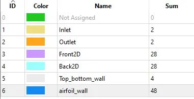
The geometry is provided with different names (inlet, outlet, front2D, back2D, top_bottom_wall, airfoil_wall) to provide boundary conditions easily.

Velocity calculations:

`Re=(rho*V*l)/mu`

Re= 200000

`rho= 1.225(kg)/m^3`

l= 0.1m

`mu=1.846e-5kg/(m*s)`

`v=(Re*mu)/(rho*l)=(200000*1.846*10^-5)/(1.225*0.1)=30.14m/s`

Case setup:

1. Parameters:

Solver= transient

Temporal type= time-based simulation

Simulation mode= full-hydrodynamic

Gas flow solver= compressible

2. Simulation time parameters:

Start time= 0s

End time= 1s

Initial time-step= 1e-5s

Minimum time-step= 1e-5s

Maximum time-step= 1s

Maximum convection CFL limit= 1

3. Regions and initialization:

Stream ID= 0

Velocity(x,y,z)= (30.14, 0, 0)

Temperature= 300K

Pressure= 101325Pa

Species= air

4. Boundary:

Inlet:

Inflow boundary condition

Velocity(x,y,z)= (30.14, 0, 0)

Temperature= 300K

Species= air

Outlet:

Outflow boundary condition

Pressure= 101325Pa

Species backflow= air

Front2D, Back2D:

2D boundary condition

Top_bottom_wall:

Slip wall boundary condition

Wall motion= stationary

Surface moement= fixed

Airfoil_wall:

No-slip wall boundary condition

Wall motion= stationary

Surface moement= fixed

5. Turbulence model used:

Part1: RNG K-epsilon, K-omega SST turbulence model

Part2: K-omega SST turbulence model

6. Base grid:

Base grid size (x, y, z)= (0.02, 0.02, 0.2)m

Fixed ebedding

Entity type= boundary

Boundary ID= airfoil_wall

Mode= sequential

Scale= 2

Embed layers= 10

Start time= 0s

End time= 10s

7. Output files:

Wall output= boundaries only

Time interval for writing 3D output data files= 0.01s.

Time interval for writing text output= 1e-5s

Time interval for writing restarting output= 0.01s

Maximum number of restarting files saved= 3

Part1:

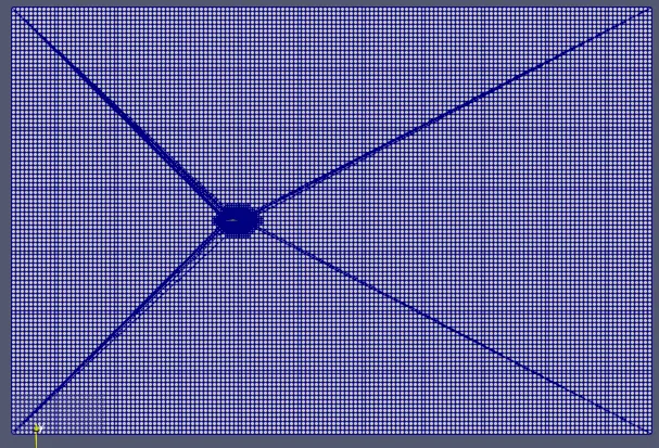
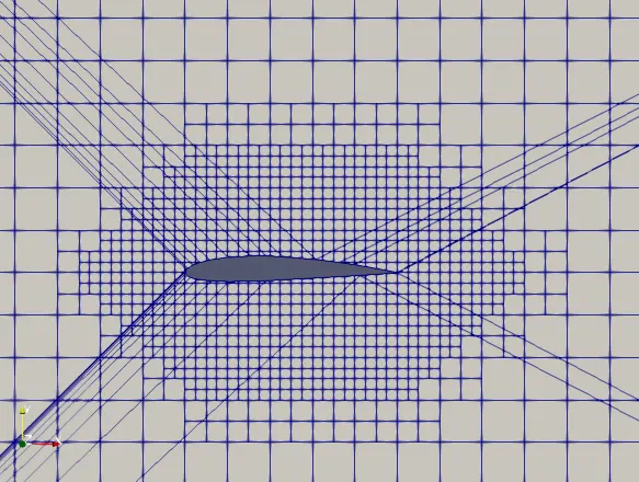
To choose the right turbulence model to perform the flow over the NACA 2412 airfoil, the simulation was performed for a given grid size and boundary conditions and different turbulence models were used and the results obtained were compared with the experimental data. The turbulence modes which give results with the least error is chosen to perform the remaining simulations at different angles of attack. A coarse mesh is used to perform this simulation to reduce the simulation time, by doing so, the simulation time is reduced but the accuracy of the solution is compromised. To improve the accuracy of the solution, the grd size must be reduced, and the embed scale can be further increased.

Angle of attack= 0 degree

Mesh:

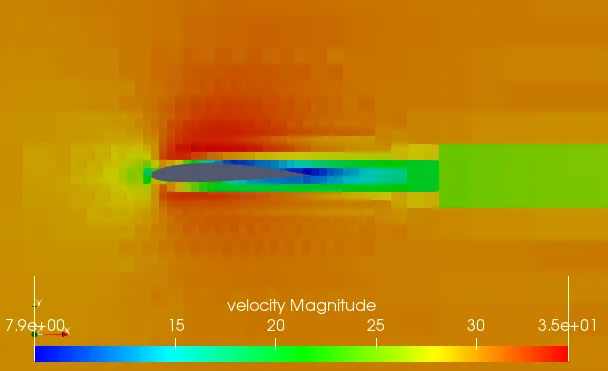
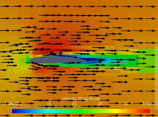
1. K-epsilon turbulence model

Velocity contours:

Pressure contours:

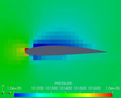
Lineplots:

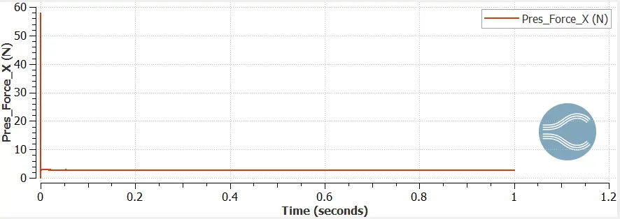
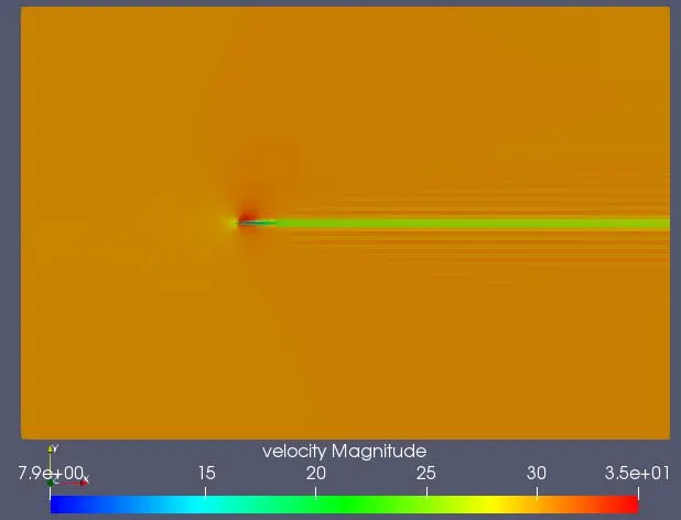
Drag force calculated as a time average from 0.9-1s is 2.7746N

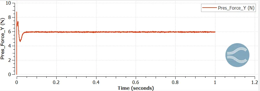
Lift force calculated as a time average from 0.9-1s is 5.934709N

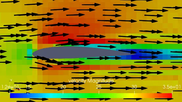
2. K-omega SST turbulence model

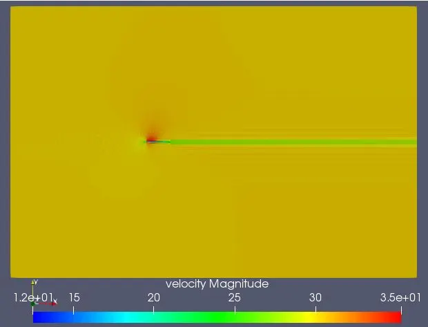
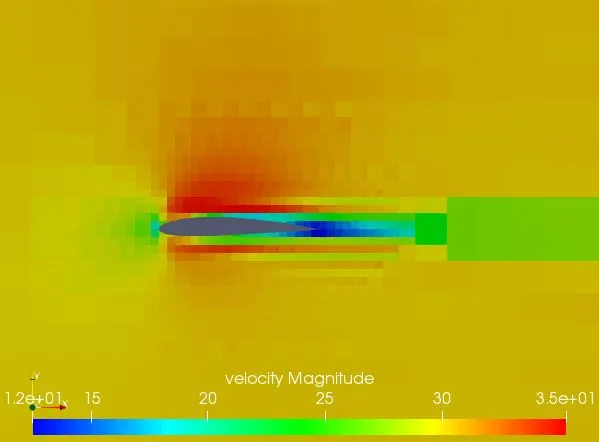
Velocity contours:

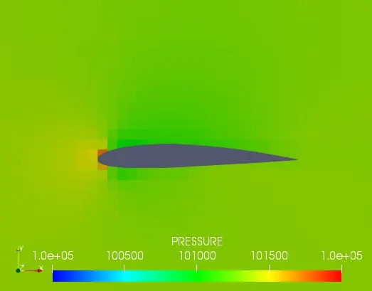
Pressure contours:

Lineplots:

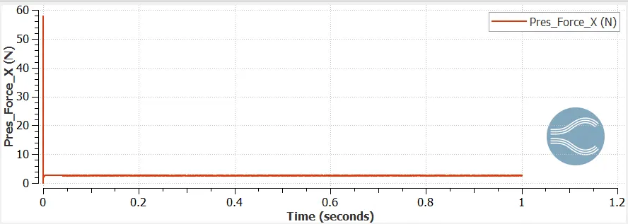
Drag force calculated as a time average from 0.9-1s is 2.565239N

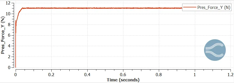
Lift force calculated as a time average from 0.9-1s is 11.0244N

Comparison of results obtained in part1:

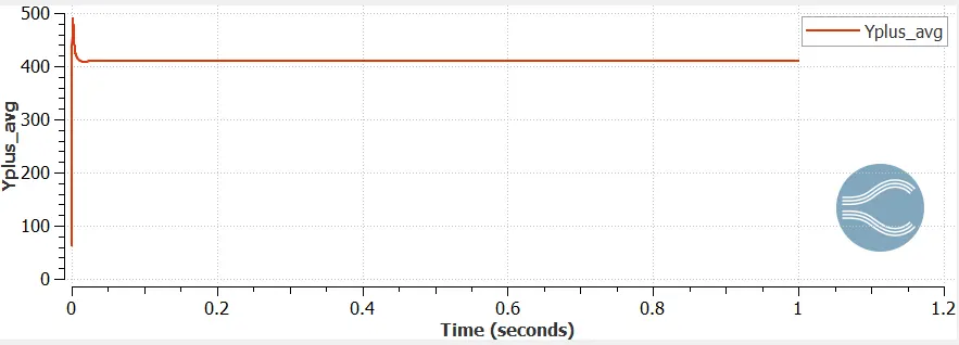
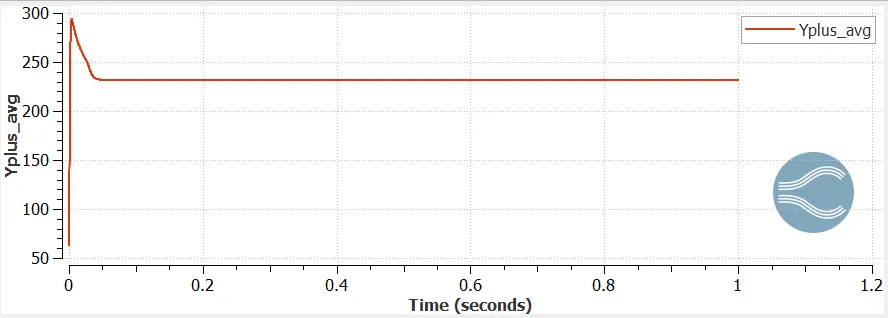
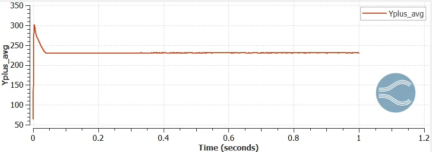
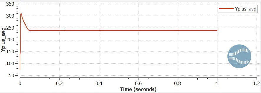
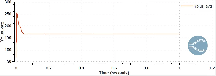
The accuracy of the solution can be improved by increasing the number of mesh elements, but this is not possible due to hardware limitations. The average Yplus value converges at around 225. Which is very high and hence the accuracy of the solution is compromised to solve the problem within a given time.

Sl. No.	Turbulence model	Lift force, N (simulated)	Coefficient of lift (Cl)	Coefficient of lift (experimental)	% error	Drag force, N (simulated)	Coefficient of drag
1	K-epsilon	5.934709	0.1066	0.20514	48.03%	2.7746	0.0498
2	K-omega SST	11.0244	0.1981	0.20514	3.43%	2.565239	0.0461

The simulated values obtained were compared with the experimental data, and since the results obtained using the K-omega SST turbulence model are more accurate, the simulations in part2 were carried out using the K-omega SST turbulece model.

[Ref: https://peer.asee.org/aerodynamic-performance-of-the-naca-2412-airfoil-at-low-reynolds-number]

Part2:

1. Angle of attack= 1 degree

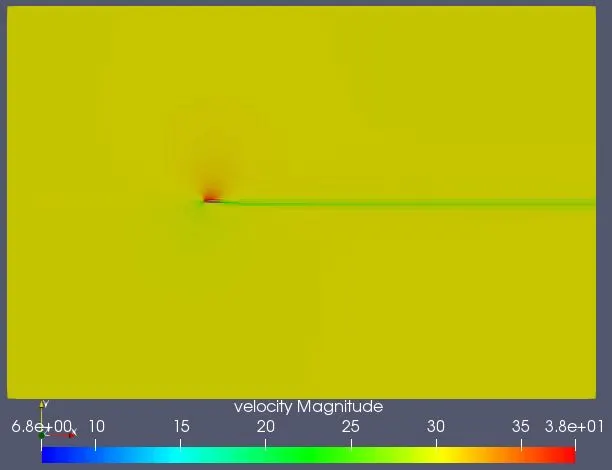
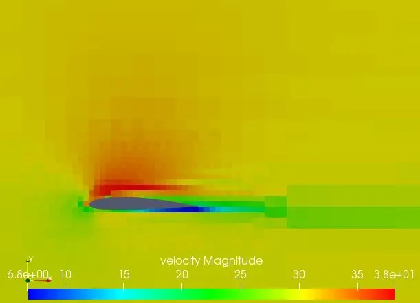
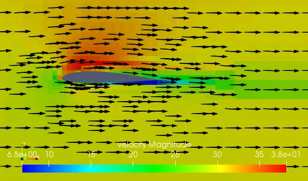
Velocity contours:

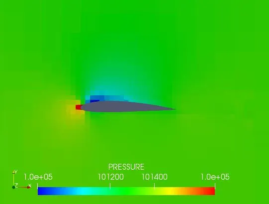
Pressure contours:

Lineplots:

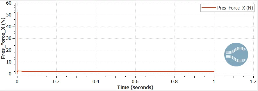
Drag force calculated as a time average from 0.9-1s is 1.962737N

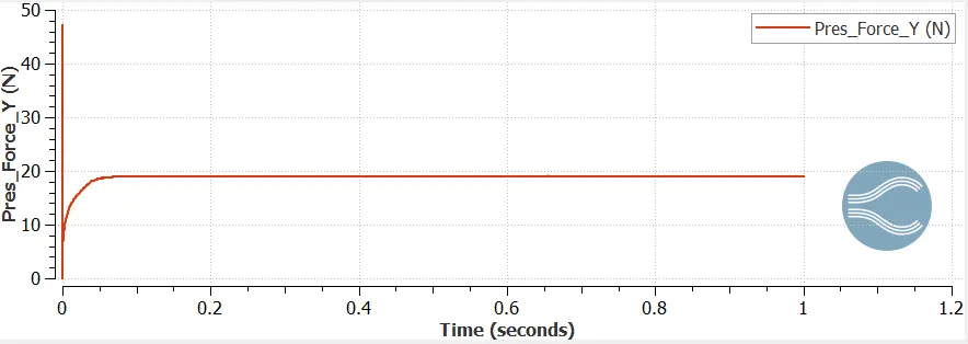
Lift force calculated as a time average from 0.9-1s is 18.98651N

2. Angle of attack= 5 degrees

Velocity contours:

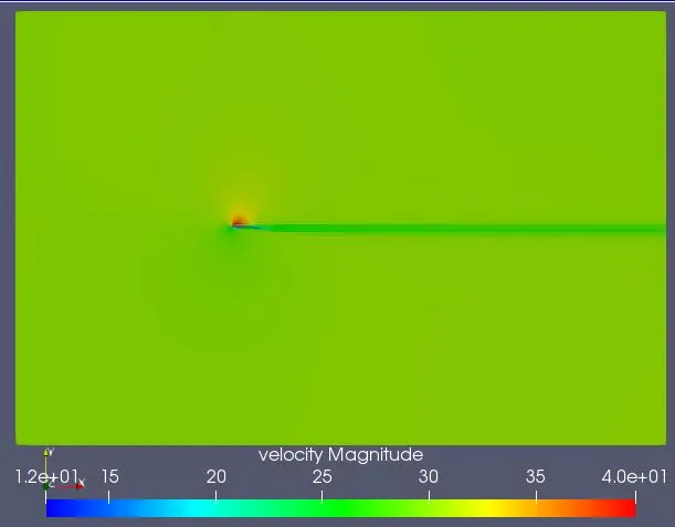
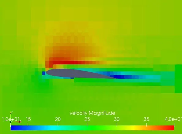
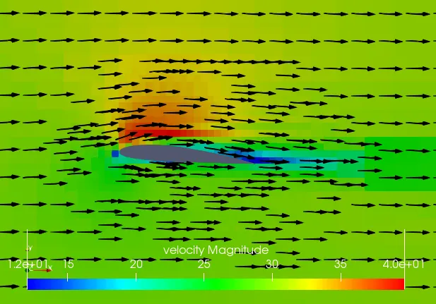
Pressure contours:

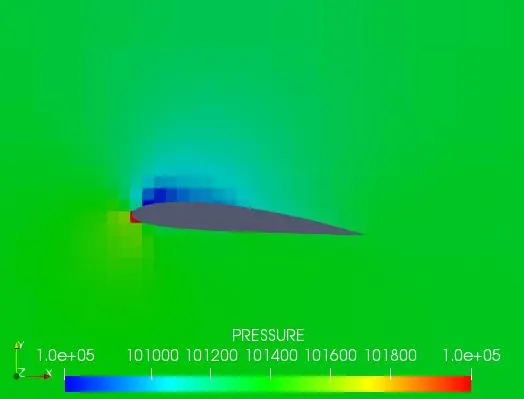
Lineplots:

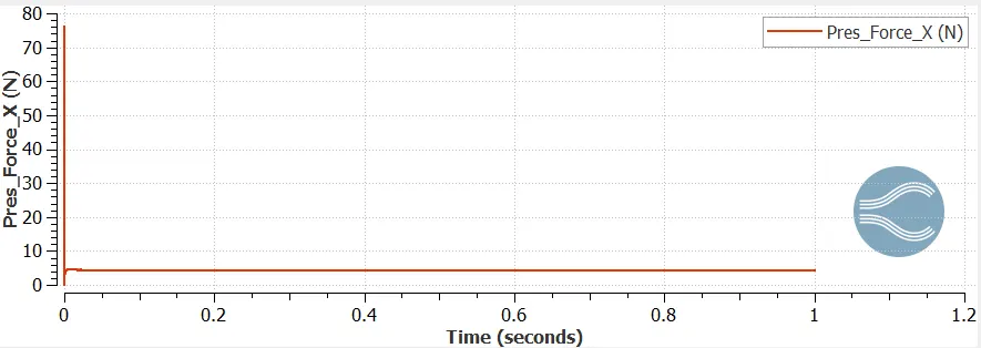
Drag force calculated as a time average from 0.9-1s is 4.313375N

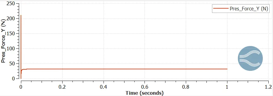
Lift force calculated as a time average from 0.9-1s is 31.85334N

3. Angle of attack= 10 degrees

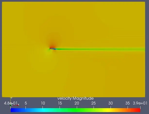
Velocity contours:

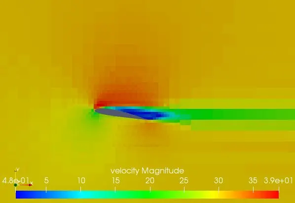
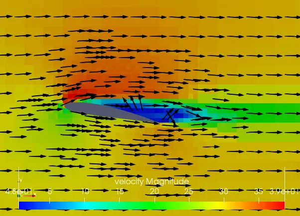
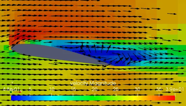
Pressure contours:

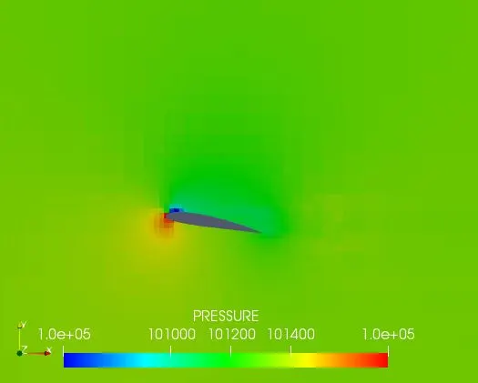
Lineplots:

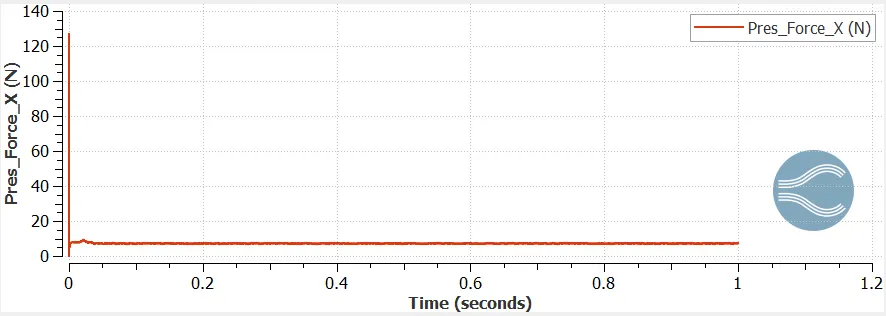
Drag force calculated as a time average from 0.9-1s is 7.15451N

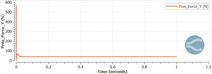
Lift force calculated as a time average from 0.9-1s is 38.60239N

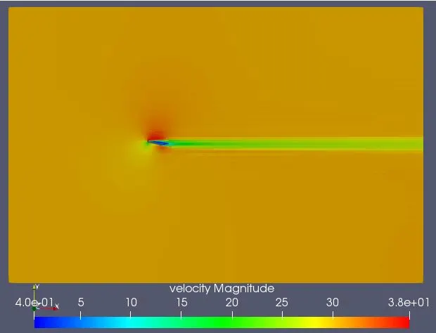
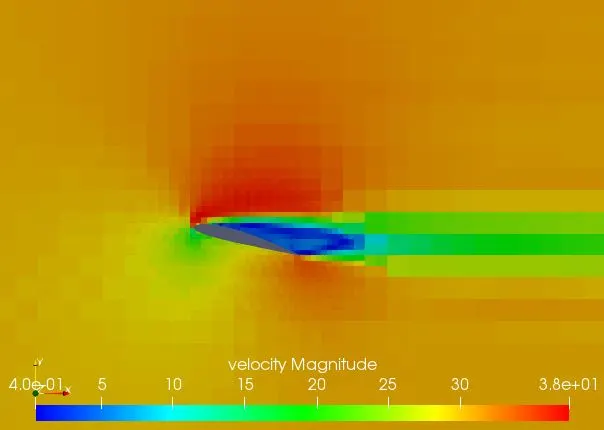
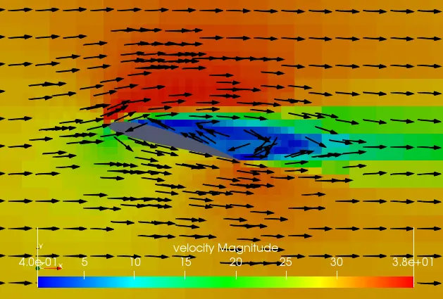
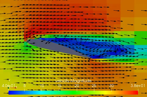
4. Angle of attack= 15 degrees

Velocity contours:

Pressure contours:

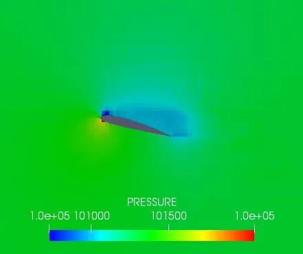
Lineplots:

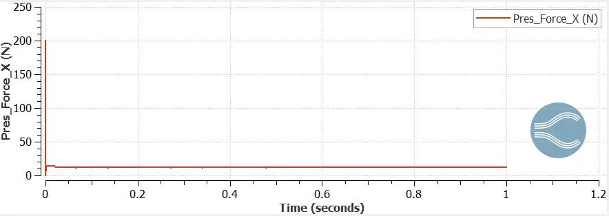
Drag force calculated as a time average from 0.9-1s is 11.9533N

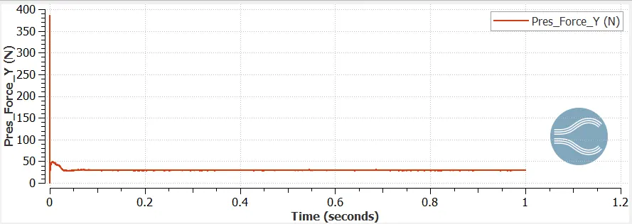
Lift force calculated as a time average from 0.9-1s is 29.40409N

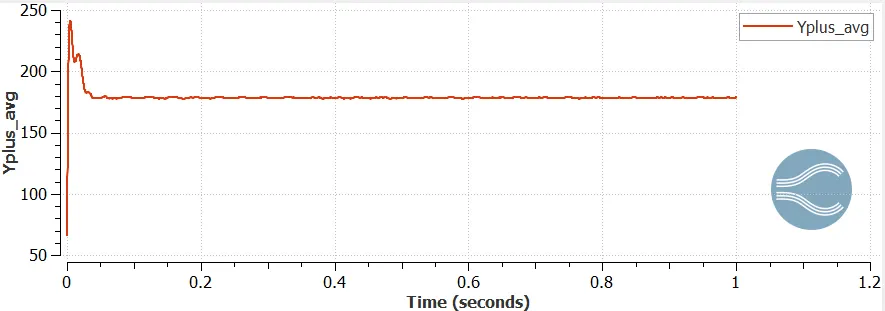
Comparison of results obtained in part2:

Lift, L= `1/2*rho*V^2*S*C_l`

Drag, D= `1/2*rho*V^2*S*C_d`

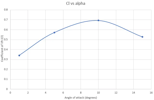
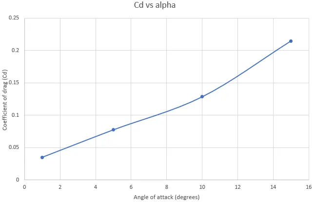
Sl. No.	Angle of attack (degrees)	Lift force, L (N)	Coefficient of lift (Cl)	Drag force, D (N)	Coefficient of drag (Cd)
1	1	18.9865	0.3412	1.9627	0.0352
2	5	31.8533	0.5724	4.3133	0.07752
3	10	38.6023	0.6937	7.1545	0.1285
4	15	29.4041	0.5284	11.9533	0.2148

Coefficient of lift vs angle of attack:

Coefficient of drag vs angle of attack:

Conclusions:

The flow analysis was performed on NACA 2412 airfoil with Reynolds number of 200000 and the following conclusions can be drawn:

1. The drag force and coefficient of drag increases with the increase in the angle of attack of the airfoil due to the increase in the frontal area
2. The lift force and coefficient of lift increases linearly with the angle of attack of the airfoil upto a point and then begins to reduce. This is due to flow the seperation occuring from the trailing edge of the airfoil.
3. As the airfoil angle of attack increases the flow remains attached to the airfoil up to a particular angle of attack, which increases the lift force and coefficient of lift of the airfoil. When the airfoil angle of attack is further increased, the flow separates, which decreases the lift force and coefficient of lift.
4. High lift devices like leading/trailing edge flaps, slats, spoilers, etc can be used to delay stall/flow separation and increase the lift produced by the wing/airfoil.
5. The accuracy of the solution obtained can be improved by reducing the mesh grid size, increasing the embed scaling, and by maintaining the value of yplus term within a certain limit for the given turbulence model.