Simulation of flow through a channel using CONVERGE CFD
Aim:
To simulate the flow of air through a 2D channel using Converge CFD.
Introduction:
The laminar flow through a square channel is a very simple problem which can be a good problem to start with learning a new CFD software. In this problem, we are simulating a laminar flow through a 2D square channel for three different mesh sizes and the obtained results are compared.
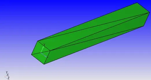
Simple geometry is created in Converge CFD and the dimensions in x, y, and z directions are 0.1, 0.01, and 0.01m respectively. The faces of the geometry are given different names(inlet, outlet, front_2d, back_2d, and top_bottom) so that the boundary conditions can be provided easily.
Case setup:
1. Mesh Sizes: (Element size along X, Y, Z axes) (in meters)
There is only one element along the Z-axis (2D simulation).
Case1: (2e-4, 2e-4, 0.01)
Case2: (1.5e-4, 1.5e-4, 0.01)
Case3: (1e-4, 1e-4, 0.01)
2. Type of simulation: Steady-state simulation with zero reactions and only air(77% N2, 23% O2) as the medium of flow.
3. Steady-state monitor properties:
a) Average velocity at the outlet
b) Average mass flow rate at the outlet
4. Boundaries:
Inlet: Inflow boundary condition with pressure inlet (100001Pa).
Outlet: Outflow boundary condition with pressure outlet (100000Pa).
Top and Bottom: Stationary, no-slip wall.
Front and Back: 2D faces.
5. Solver properties:
Details: 2 minimum iterations and 20 max iterations per cycle. Tolerance = 0.001
Minimum Cycles = 0
Maximum Cycles = 15000
Minimum time step = 1e-9 sec
Maximum time step = 1 sec
Maximum convection CFL limit(final stage)= 0.5
Results:
Case1: mesh grid size= 2e-4m
mesh:
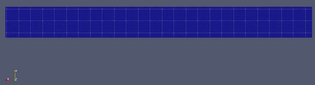
Total number of mesh elements generated= 25000
Velocity contours:
Pressure contours:
Line plots:
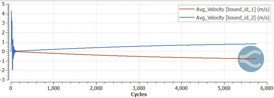
Average velocity:
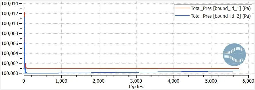
Total pressure:
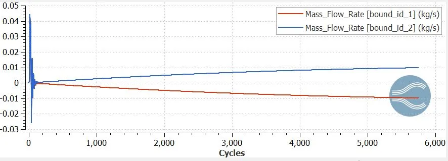
Mass flow rate:
Cell count:
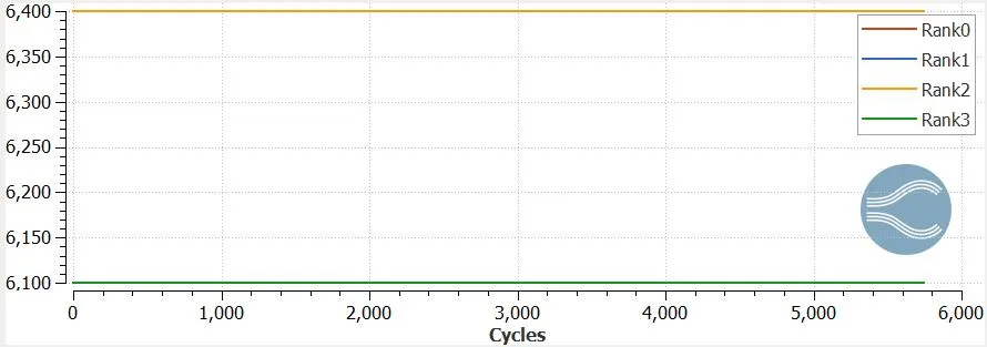
Total number of cells handled by Rank0 and Rank3 processors= 6100
Total number of cells handled by Rank1 and Rank2 processors= 6400
Case2: mesh element size= 1.5e-4m
Mesh:
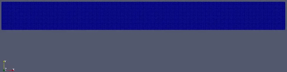
Total number of mesh elements generated= 45420
Velocity contours:
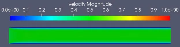
Pressure contours:
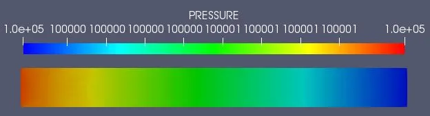
Line plots:
Average velocity:
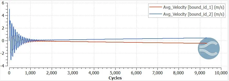
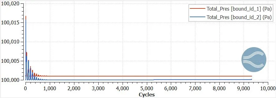
Total pressure:
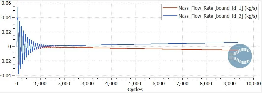
Mass flow rate:
Cell count:
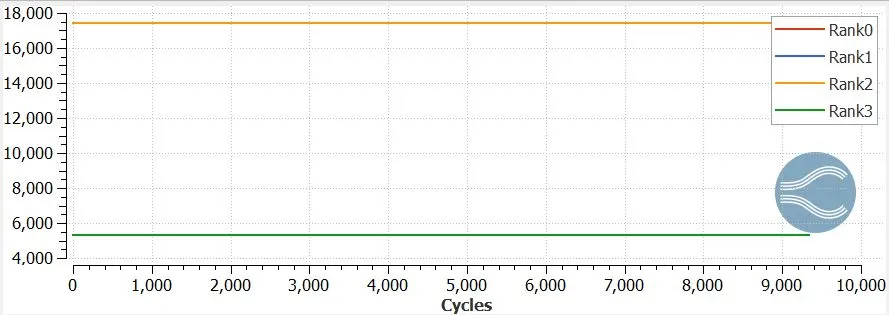
Total number of cells handled by Rank0 and Rank3 processors= 5302
Total number of cells handled by Rank1 and Rank2 processors= 17408
Case3: mesh element size= 1e-4m
Mesh:
Total number of mesh elements generated= 100000
Velocity contours:
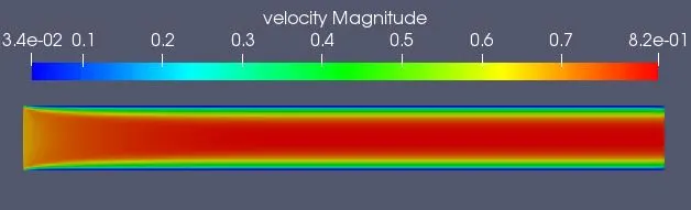
Pressure contours:
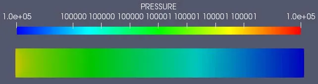
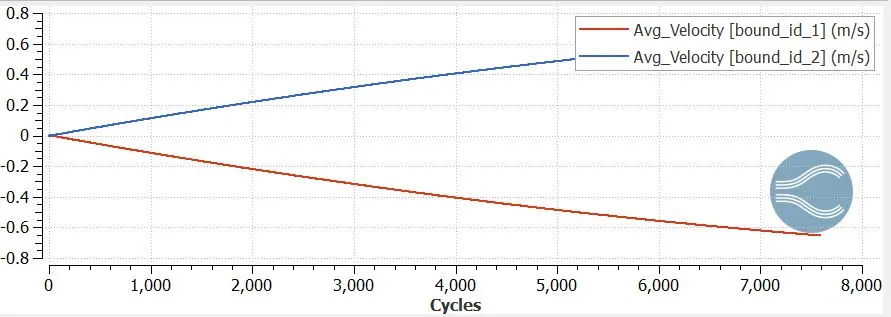
Line plots:
Average velocity:
Total pressure:
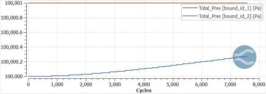
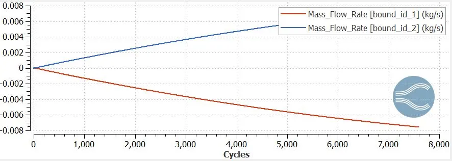
Mass flow rate:
Cell count:
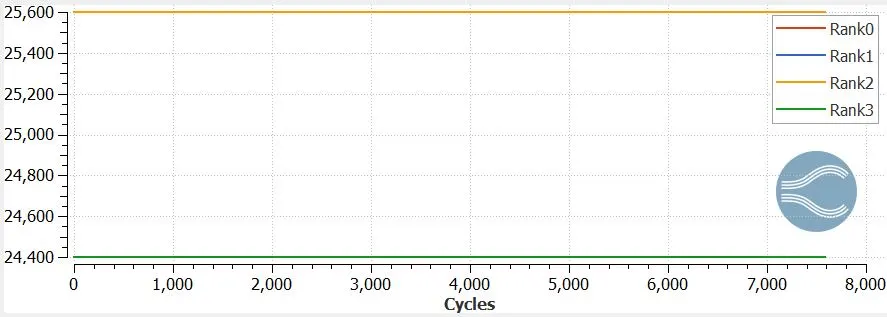
Total number of cells handled by Rank0 and Rank3 processors= 24400
Total number of cells handled by Rank1 and Rank2 processors= 25600
Conclusions:
Though the simulation was performed on the same geometry with the same boundary and initial conditions, the results obtained in all three cases is slightly different.
- With the increase in the cells the solution becomes more accurate but the computation time increases considerably. Hence, the problem must be studied thoroughly before performing the simulation and it must be decided how much are we willing to compromise the accuracy of the solution to save resources.
- Using multiple processors reduces the computation time since the cells are distributed among them.
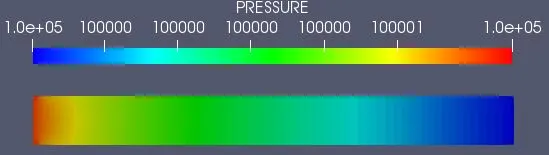
- The pressure at the outlet is higher than that at the inlet. Since fluids move from the region of higher pressure to the region of lower pressure, the velocity and mass flow rate is higher at the outlet than at the inlet.
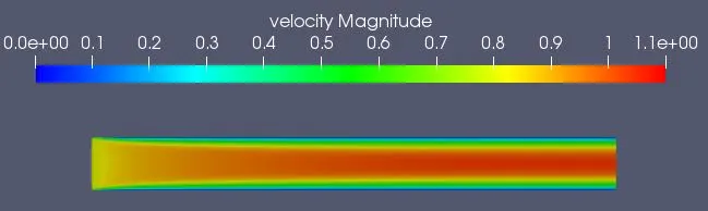
- Near the inlet, the velocity magnitude remains almost constant between the walls. The boundary conditions at the wall is stationary no-slip. Hence at the surface of the wall, the velocity magnitude is zero and is the highest in middle of the walls. In the fully developed region, the velocity magnitude of the fluid is the highest at the center of the two walls.