Conjugate Heat Transfer (CHT) simulation using Converge CFD

The term conjugate heat transfer(CHT) is used to describe processes that involve variations of temperature within solids and fluids, due to thermal interaction between the solids and fluids. The exchange of thermal energy between the two physical bodies is called the study of Heat Transfer. The rate of transferred heat is directly proportional to the temperature difference between the bodies. A typical example is the heating or cooling of a solid object by the flow of air in which it is immersed and some other example includes conduction through solids, free and forced convection in the gases/fluids, and thermal radiation.

Conjugate heat transfer corresponds with the combination of heat transfer in solids and heat transfer in fluids. In solids, conduction often dominates whereas, in fluids, convection usually dominates. Efficiently combining heat transfer in fluids and solids is the key to designing effective coolers, heaters, or heat exchangers. Forced convection is the most common way to achieve a high heat transfer rate. In some applications, the performances are further improved by combining convection with phase change (for example liquid water to vapor phase change).

Heat transfer in solids and heat transfer in fluids are combined in the majority of applications. This is because fluids flow around solids or between solid walls and because solids are usually immersed in a fluid. The fluid flow and heat transfer problems can be tightly coupled through the convection term in the energy equation and when physical properties are temperature-dependent. While analytical solutions exist for some simple problems, we must rely on computational methods to solve most industrially relevant applications.

Super-cycle modeling:

The internal combustion engine industry is moving toward simulating the entire system rather than independent components. Conjugate heat transfer (CHT)—the simultaneous prediction of heat transfer in both the fluid and solid portions of the domain—is of critical importance in a full-engine simulation. The accuracy of the predicted combustion in the cylinder is dependent on the temperature boundary conditions in the cylinder. By considering heat transfer in the metal components (e.g., the cylinder head, liner, piston, etc.) in the simulation, the cylinder wall no longer has a user-specified temperature but instead has temperatures predicted as part of the system simulation. This makes the overall simulation results more predictive by reducing the dependence on boundary conditions.

There are several challenges when solving the fluid and solid domains together. The largest challenge to overcome is the difference in time-scales associated with the fluid and solid. In general, the heat transfer in the solid occurs more slowly than the convective and diffusive time-scales dictated by the fluid flow in the cylinder. For example, when you start a car in cold temperatures, combustion occurs almost instantly while the coolant takes minutes (thousands of cycles) to reach a steady-state temperature. This disparity in time-scales is problematic for CFD simulation because each cycle can be computationally expensive.

CONVERGE offers an alternative approach called super-cycling for overcoming the time-scale disparity. In super-cycling, the fluid solver is frozen periodically while the heat transfer in the solid is allowed to progress to steady-state. CONVERGE solves the fluid and solid phases in the same simulation without requiring you to stop and restart the simulation. Super-cycling significantly reduces the computational cost of the CHT simulation.

Yplus:

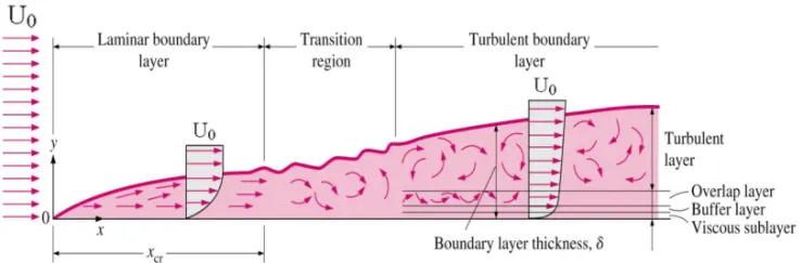
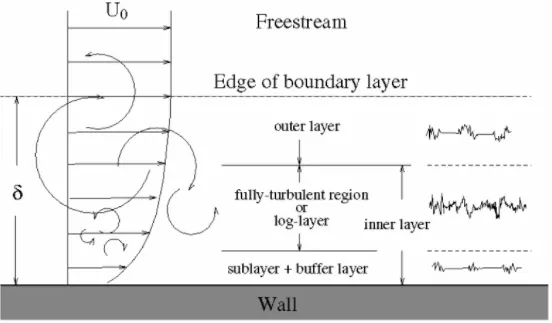
The behavior of the flow near the wall is a complicated phenomenon and to distinguish the different regions near the wall the concept of wall yplus has been formulated. Thus yplus is a dimensionless quantity and is the distance from the wall measured in terms of viscous lengths.

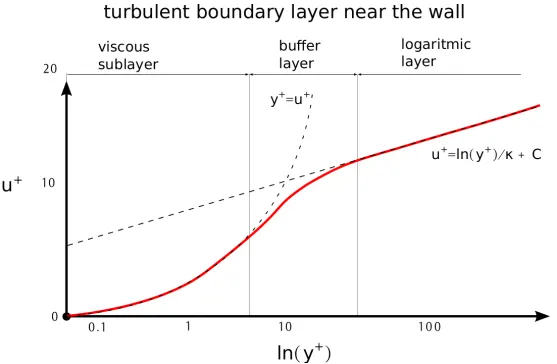
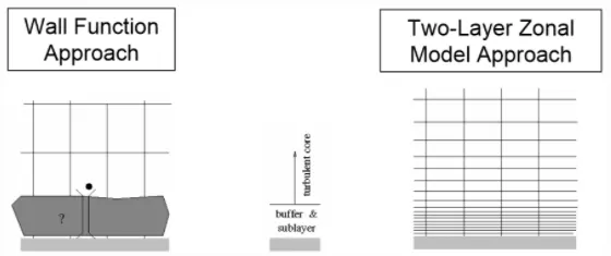
The yplus value denotes the point where the yplus vs uplus curve we are with respect to the cell size. It is undesirable to have a cell size that leads to a y+ of between 10 to 30 since the modeling of flows transitioning from laminar to turbulent is not easy and is still being researched. Due to this fact, it is better to have a yplus of less than 10 meaning the flow will be at the laminar region or have a yplus of greater than 30 and use wall functions and still achieve results. The yplus value can be used as a marker based on which we can decide on the base grid size and make a decision based on the computing power as to whether the grid needs to be refined further or coarsened.

Geometry:

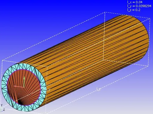
The geometry setup consists of an aluminum pipe of circular cross-section with an outer and inner radius of 0.02m and 0.015m respectively. The length of the pipe is taken as 0.2m. The fluid flowing through the pipe is air. The faces of the geometry are given different names(inlet, outlet, solid_side, solid_outer_wall, and interface_wall) so that the boundary conditions can be provided easily.

Initial conditions to maintain inlet Reynolds number as 7000

`Re=(rho*V*D)/mu`

Re= 7000

`rho=` density of air= 1.225 Kg/m^3

D= hydraulic dameter= 0.03m

`mu=`dynamic viscosity of air= 1.846e-5 Kg/ms

`V= (Re*mu)/(rho*D)=(7000*1.846*10^-5)/(1.225*0.03)=3.516m/s`

Case setup:

1. Mesh size:

Three cases:

1. 0.004m (In all three coordinate axes) (baseline mesh)

2. 0.003m (In all three coordinate axes)

3. 0.002m (In all three coordinate axes)

2. Type of simulation: Transient-state simulation with zero reactions and only air(77% N2, 23% O2) as the medium of flow.

3. Regions and initialization:

Fluid region:

Stream ID= 0

Species= O2, N2

Solid region:

Stream ID= 1

Species= Aluminum

4. Boundaries:

The boundaries are defined in solid and fluid regions as follows

Fluid region= inlet, outlet

Solid region= solid_outer_wall, solid_side

Inlet: Inflow boundary condition with velocity inlet (V(z)= 3.5m/s)

Outlet: Outflow boundary condition with pressure outlet (101325Pa)

Solid_outer_wall: Stationary wall with slip boundary condition, temperature (Heat flux= -10000W/m^2)

Solid_side: Stationary wall with slip boundary condition

Interface_wall:

Forward boundary= fluid region, velocity and temperature boundary condition= law of wall

Reverse boundary= solid region, velocity boundary conditon= slip, temperature boundary condition= specified value

5. Turbulence model used:

RNG k-epsilon turbulence model

6. Super-cycle modeling:

Begin storing super-cycle data= 0.05s

Solid side heat transfer solver= Steady-state solver

Time length for each cycle stage= (Run for three cases using a refined mesh of mesh size 2mm)0.01, 0.02, 0.03

Total number of stages= 1

Conduction CFL number= 100

Sensible internal energy(SIE) tolerence= 1e-7

SIE relaxation factor for super-cycle= 1.4

Output points= (Provide coordinates of one point inside the solid region)

Grid independence test:

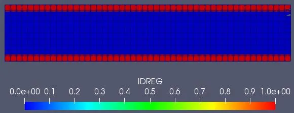
The baseline mesh(grid size= 0.004m) is generated on the given geometry taking the time length for each super-cycle stage as 0.01s. The same simulation is performed for two more cases with a refined mesh(grid sze= 0.003m, 0.002m). If the solution obtained using the coarser mesh is very close to the solution obtained using the refined mesh, ie, within a certain tolerance limit, then the coarser mesh is said to be grid-independent, and any further simulations can be performed using the coarser mesh. By doing so, the problem is solved faster without compromising much on the solution accuracy.

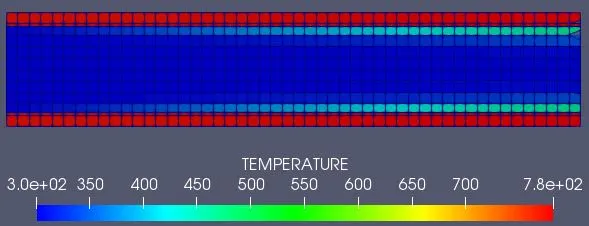
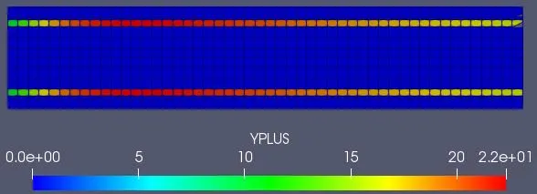
Case1: grid size= 0.004m (baseline mesh)

Mesh:

Temperature contours:

Yplus contours:

Cell count:

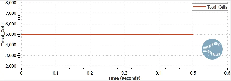
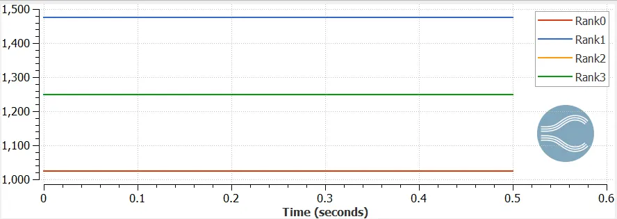
Total number of cells generated= 5000

Cell distribution among 4 processors

Rank0= 1025

Rank1= 1475

Rank2, Rank3= 1250

Case2: grid size= 0.003m

Mesh:

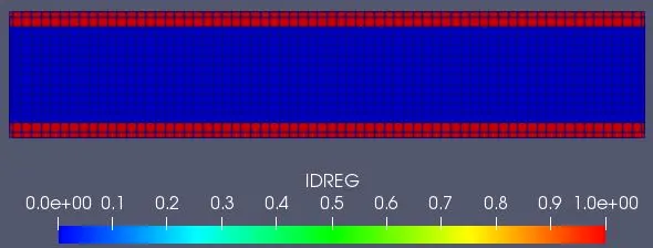
Temperature contours:

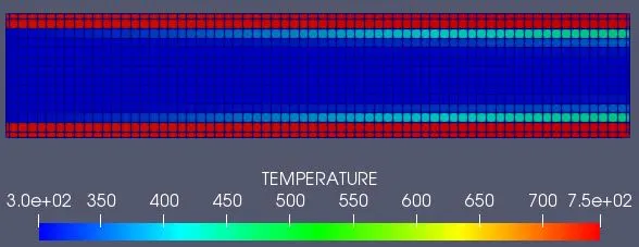
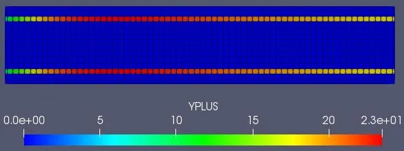
Yplus contours:

Cell count:

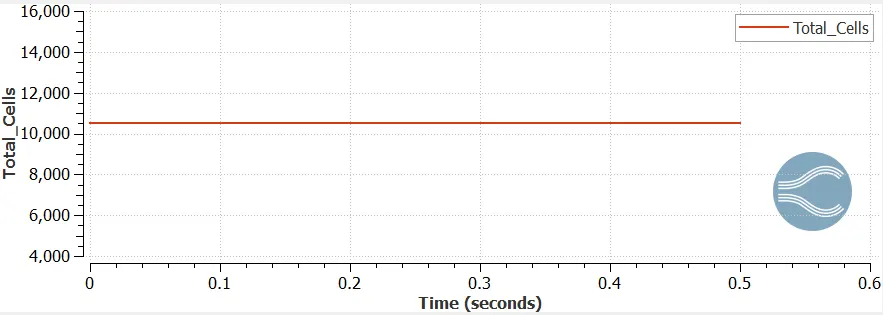
Total number of cells generated= 10496

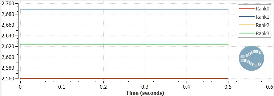
Cell distribution among 4 processors

Rank0= 2560

Rank1= 2688

Rank2, Rank3= 2624

Case3: grid size= 0.002m

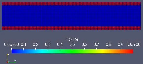
Mesh:

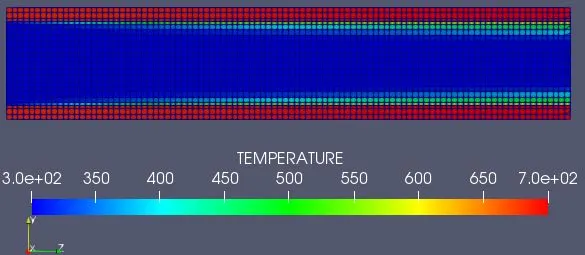
Temperature contours:

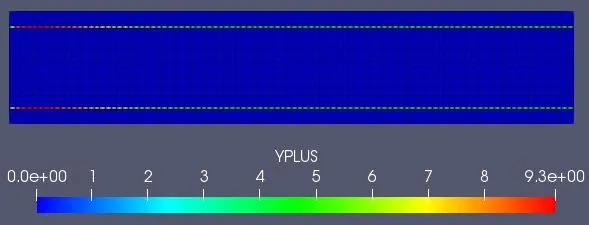
Yplus contours:

Cell count:

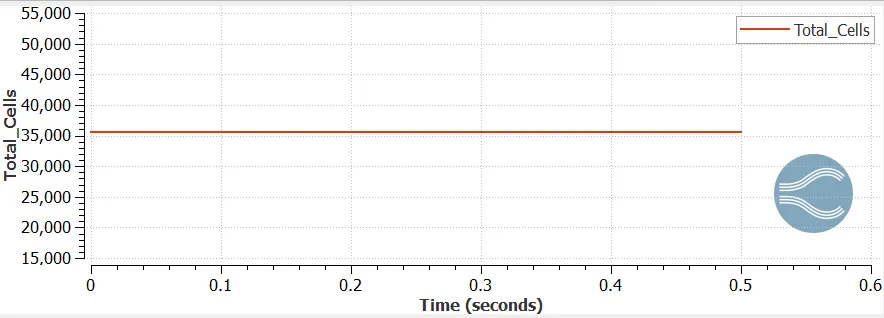
Total number of cells generated= 35600

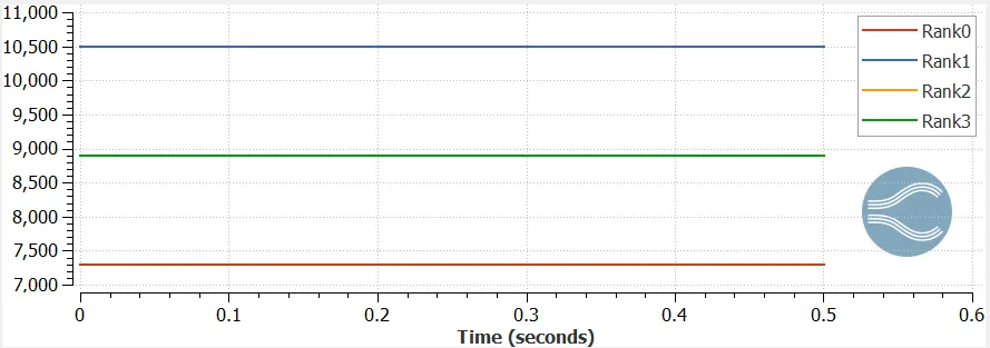
Cell distribution among 4 processors

Rank0= 7298

Rank1= 10502

Rank2, Rank3= 8900

Effet of super-cycle stage interval:

To simulate the effect of the super-cycle stage interval, the CHT analysis was run for three cases of super-cycle stage interval, ie, 0.01s, 0.02s, and 0.03s using the geometry with the mesh grid size of 0.002m.

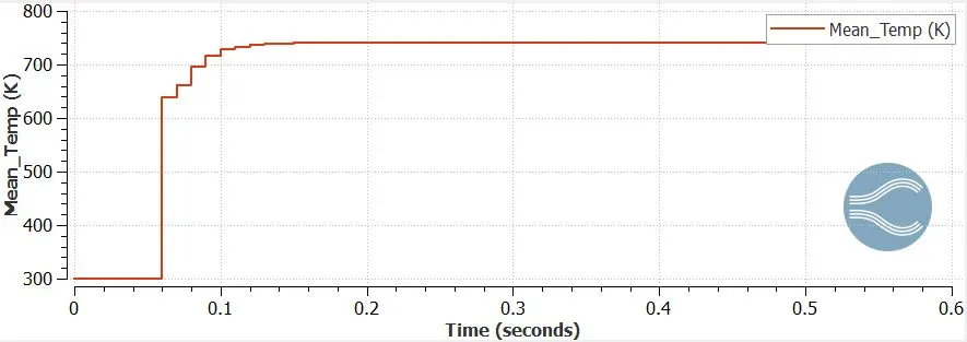
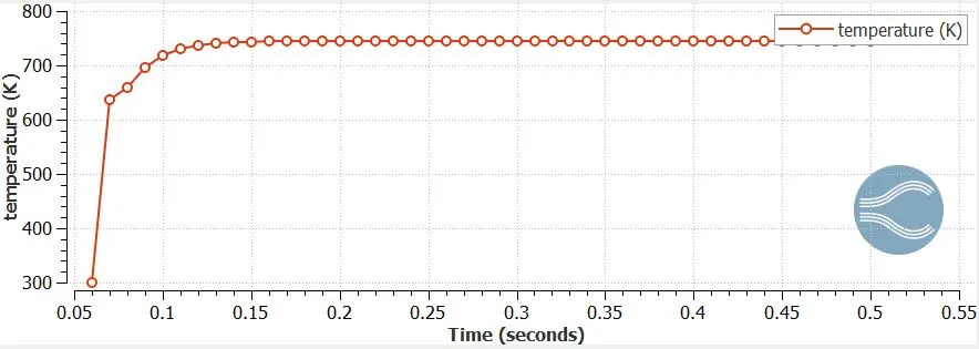
Case1: Supercycle stage interval= 0.01s

Mean temperature at the output point:

Temperature of the solid domain after each super-cycle stage:

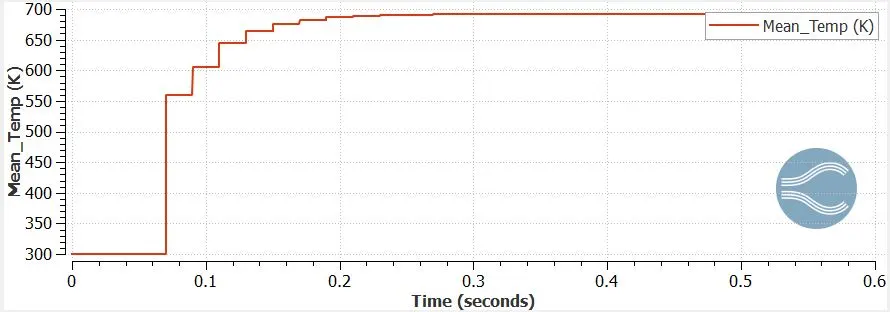
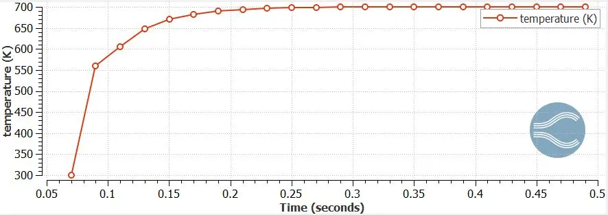
Case2: Supercycle stage interval= 0.02s

Mean temperature at the output point:

Temperature of the solid domain after each super-cycle stage:

Case3: Supercycle stage interval= 0.03s

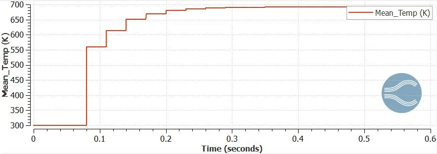
Mean temperature at the output point:

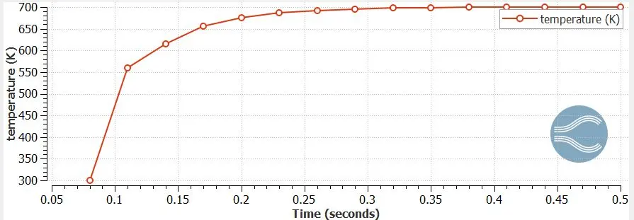
Temperature of the solid domain after each super-cycle stage:

Conclusions:

1. The simulation time to solve the problem using the baseline mesh of grid size 0.004m is 507.786s, which is comparatively lower than the simulation time to solve the refined mesh taking 0.01s as the super-cycle stage interval. The time taken to solve the problem using the grid size of 0.003m and 0.002m is 1348.02s and 4408.58s respectively. Also, the simulation time increases marginally as the super-cycle stage interval is increased. The simulation time for solving the problem with 2mm mesh grid size and the super-cycle stage interval of 0.01s, 0.02s, and 0.03s is 4408.58s, 4449.105s, and 4934.772s respectively.
2. As the mesh is refined, the maximum value of the Yplus term also reduces. For the esh grid sizes of 0.004m, and 0.003m, the Yplus term varies from 0 to ~23. But when the grid size is further reduced to 0.002m, the ypus term also reduces to ~9.3.
3. The smaller the super-cycle stage interval taken, the faster is the convergence to a steady-state value. The temperature at the supercycle output point converges to almost 700K

References:

1. https://www.depusa.com/solutions/services/cae-services/conjugate-heat-transfer/#:~:text=The%20term%20conjugate%20heat%20transfer,between%20the%20solids%20and%20fluids.
2. https://convergecfd.com/benefits/conjugate-heat-transfer
3. https://www.learncax.com/knowledge-base/blog/by-category/cfd/basics-of-y-plus-boundary-layer-and-wall-function-in-turbulent-flows