Simulation of Prandtl Meyer Shock using Converge CFD

Aim:

To simulate the Prandtl-Meyer shock wave (expansion fan) over a sharp edge for different values of sub-grid scale(SGS) criterion and draw suitable conclusions.

Theory:

For solving the steady-state flow appropriate boundary conditions are needed. It is one of the required components of the mathematical model. On the other hand, for solving transient flow, appropriate initial conditions are also required. Types of boundary conditions that are typically used to solve shock flow problems are:

1. Dirichlet boundary conditions:

The Dirichlet boundary condition is a type of boundary condition, which specifies the values that a solution needs to take along the boundary of the domain.

2. Neumann boundary conditions:

The Neumann boundary condition is a type of boundary condition, which specifies the values in which the derivative of a solution is applied within the boundary of the domain. Pressure outlet boundary conditions require the specification of a static (gauge) pressure at the outlet boundary. The value of the specified static pressure is used only while the flow is subsonic. If the flow is supersonic, the specified pressure will no longer be used, pressure will be extrapolated from the flow in the interior. This means that Neumann Boundary Conditions which say that the outlet condition is dependent on the initial conditions of the flow need to be used in this case, which will derive the value of pressure from the initial conditions.

3. Mixed boundary conditions:

The mixed boundary conditions require the solution to satisfy a Dirichlet or Neumann boundary condition in a mutually exclusive way on disjoint parts of the boundary.

Shock wave:

A shock wave is a type of propagating disturbance that moves faster than the local speed of sound in the medium. A shock wave carries energy and can propagate through a medium that is characterized by an abrupt, nearly discontinuous, change in pressure, temperature, and density of the medium. the energy and speed of a shock wave alone dissipate relatively quickly with distance. When a shock wave passes through matter, energy is preserved but entropy increases. This change in the matter's properties manifests itself as a decrease in the energy which can be extracted as work, and as a drag force on supersonic objects. The shock waves are strongly irreversible processes.

Prandtl Meyer expansion fan:

It is a centered expansion process that occurs when a supersonic flow turns around a convex corner. The fan consists of an infinite number of Mach waves, diverging from a sharp corner. When a flow turns around a smooth and circular corner, these waves can be extended backward to meet at a point. Each wave in the expansion fan turns the flow gradually (in small steps). The theory was described by Theodor Meyer on his thesis dissertation in 1908, along with his advisor Ludwig Prandtl. This theory was named after them.

Geometry:

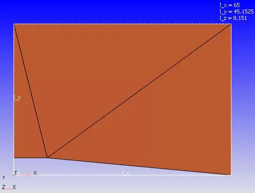
To simulate the Prandtl-Meyer expansion fan, a geometry is greater as shown above. Since we are performing a 2D analysis, the dimension of the generated geometry in the z-direction is given randomly and ignored. The faces of the geometry are given different names(inlet, outlet, front_2d, back_2d, and top_bottom) so that the boundary conditions can be provided easily.

Case setup:

1. mesh sizes

The mesh element size in all three coordinate axes is taken as 0.8m

2. Type of simulation: Steady-state simulation with zero reactions and only air(77% N2, 23% O2) as the medium of flow.

3. Steady-state monitor properties:

a) Average velocity at the outlet

b) Average mass flow rate at the outlet

c) Average temperature at the outlet

4. Boundaries:

Inlet: Inflow boundary condition with velocity inlet (V(x)= 680m/s).

Outlet: Outflow with Neumann boundary conditions for pressure and velocity.

Top and Bottom: Stationary, slip wall.

Front and Back: 2D faces.

5. Initial conditions:

Velocity (x)= 680m/s

Temperature= 300K

Pressure= 101325Pa

6. Solver properties:

Start time= 0 cycles

End time = 25000 cycles

Initial time-step= 1e-6s

Minimum time step= 1e-6s

Maximum time step= 1s

Maximum convection CFL limit(final stage)= 0.5

7.Turbulence model:

RNG K-epsilon turbulence model

8. Adaptive mesh refinement:

Minimum cells= 1

Maximum cells= 200000

Embedding type: temperature sub-grid scale(SGS) criterion

Maximum embedding level= 2

Sub-grid criterion (3 cases)= 0.05K, 0.01K, 0.1K

Solution:

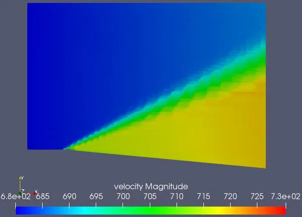
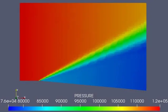
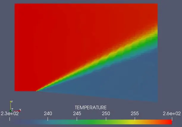
Case1: Sub-grid scale(SGS) criterion= 0.05K

Mesh:

Velocity contours:

Pressure contours:

Temperature contours:

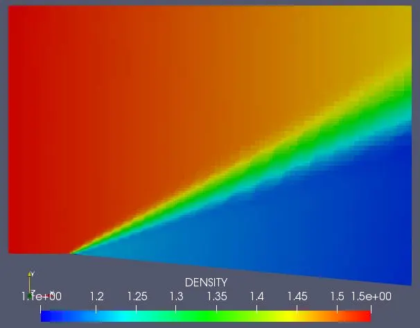
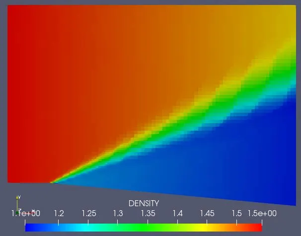
Density contours:

Cell count:

Case2: Sub-grid scale(SGS) criterion= 0.01K

Mesh:

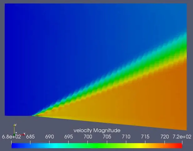
Velocity contours:

Pressure contours:

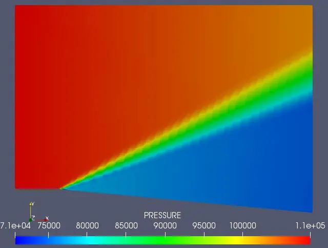
Temperature contours:

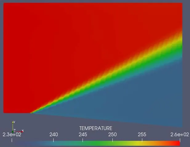
Density contours:

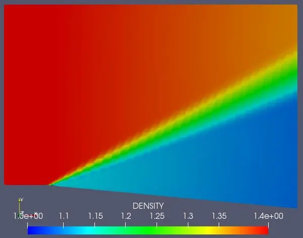
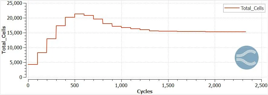
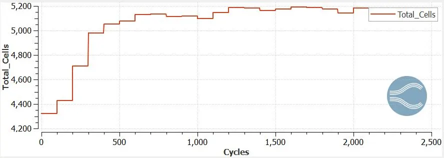
Cell count:

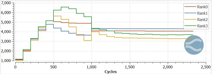
Case3: Sub-grid scale(SGS) criterion= 0.1K

Mesh:

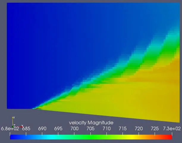
Velocity contours:

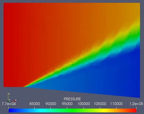
Pressure contours:

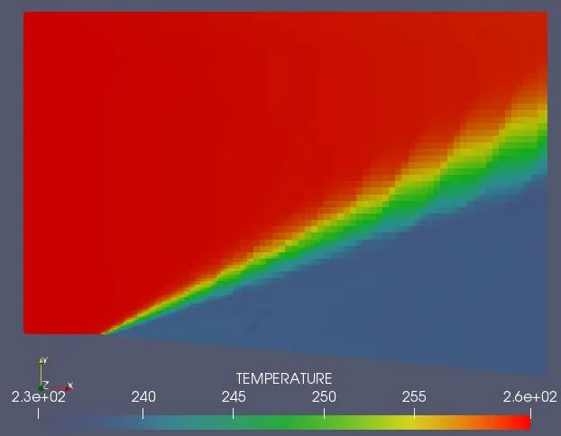
Temperature contours:

Density contours:

Cell count:

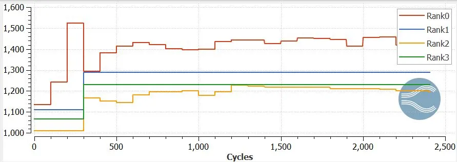
Conclusions:

1. When air with supersonic speed flows over a convex sharp edge, it leads to the formation of a series of shock waves, which tends to turn the fluid towards the void. These waves diverge from the sharp corner and are also called Mach waves.
2. Here, the simulation was performed for flow Mach number of 2 (flow velocity= 680m/s), for three different temperature sub-grid scale (SGS) criterion of 0.05K, 0.01K, and 0.1K. In all the cases, the velocity, and hence the flow Mach number downstream the sharp edge decreases, whereas, the static pressure, temperature, and density downstream the sharp edge decreases.
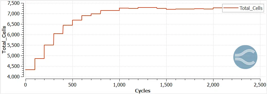
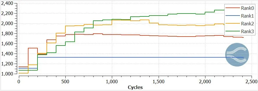
3. The lower the temperature sub-grid scale (SGS) criterion provided, the higher is the number of cells/grids generated, and hence the higher the computation time. But, providing higher values of temperature sub-grid scale (SGS) will generate a lesser number of cells but will reduce the accuracy of the obtained solution. By providing lower values of this parameter will increase the accuracy of the obtained solution but the computation time and hence resources spent will be excessive. Hence it a good practice to solve an engineering problem as quickly as possible without compromising much on the solution accuracy.
4. In this case, the temperature sub-grid scale criterion of 0.1K is too high and hence may not be accurate. On the other hand 0.01Kis too low which takes a comparatively longer time to solve. The temperature SGS of 0.05K may be optimal to be used to solve this problem.