Simulation of mixing efficiency of air
Aim:
To set up steady-state simulations to compare the mixing effectiveness with hot inlet temperature 360C and the Cold inlet temperature 190C using the k-epsilon and k-omega SST model for the first case, and based on the judgment more suitable model is used for further cases.
- Case 1
- Short mixing tee with a hot inlet velocity of 3m/s.
- Momentum ratio of 2, 4.
- Case 2
- Long mixing tee with a hot inlet velocity of 3m/s.
- Momentum ratio of 2, 4.
Formulas:
Momentum ratio = velocity at cold inlet / velocity at hot inlet
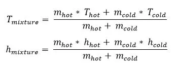
Analytical calculations:
The temperature of hot air= 360C
The temperature of cold air= 190C
The velocity of hot air= 3m/s
The diameter of cold air inlet pipe= 17mm
The diameter of hot air inlet pipe= 34mm
1) Momentum ratio= 2
The velocity of cold air= 6m/s
`T_(mixture)=((3*(pi)/4*34^2*36)+(6*(pi)/4*17^2*19))/((pi/4)*((3*34^2)+(6*17^2)))=30.33`
2) Momentum ratio= 4
The velocity of cold air= 12m/s
`T_(mixture)=((3*(pi)/4*34^2*36)+(12*(pi)/4*17^2*19))/((pi/4)*((3*34^2)+(12*17^2)))=27.5`
Case 1: Analysis of short mixing tee
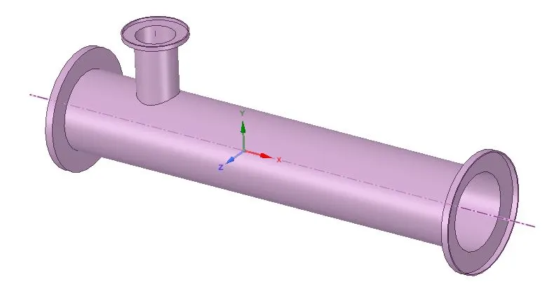
The geometry consists of a pipe with a hydraulic diameter of 34mm, to which another pipe of diameter 17mm is attached. The temperature of the air entering the first inlet is of 36-degree celsius, and the temperature of the air entering from the second inlet is 19-degree celsius. The length of the pipe is 192mm.
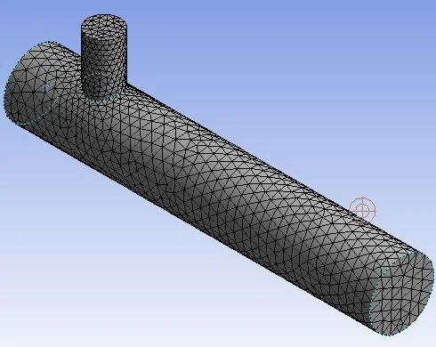
Since we are not interested in the structural analysis of the pipe and we are interested only in the fluid analysis, the volume is extracted from the above geometry, and meshing is done on the fluid by suppressing the solid geometry so that no mesh elements are generated on the pipe. Here tetrahedral meshing is used, with the element size being 0.005m. Once the meshing is done there will be a total of 14197 mesh elements for the given geometry.
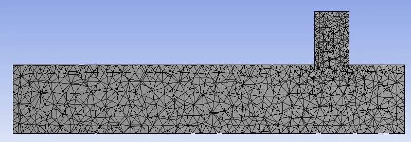
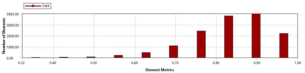
The quality of the mesh is checked, and since the majority of the mesh elements have mesh quality greater than 50%, and there are no mesh elements with mesh quality of less than 30%, the mesh is considered suitable to perform the fluent simulations.
1) Momentum ratio= 2
For a momentum ratio of 2 and with the velocity of hot air at 3m/s, the velocity of chilled air should be 6m/s. This problem is solved using the K-epsilon and the K-omega SST turbulence model, and comparisons are done between these two models.
1.1) Turbulence model used: K-epsilon
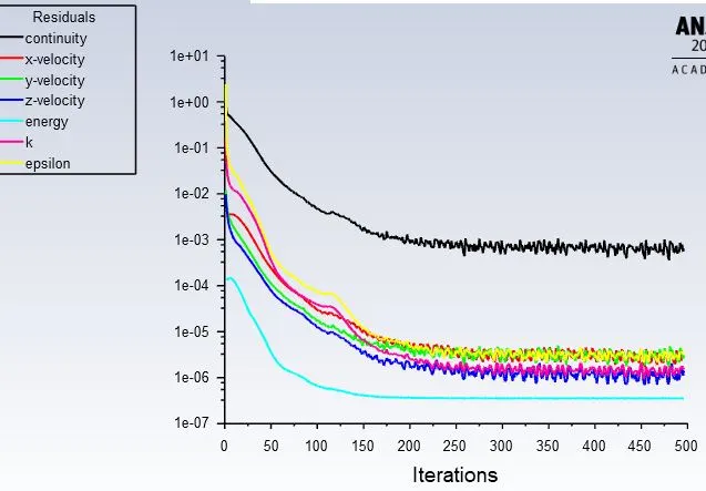
Residuals are a function of the error in the model. The higher the residual, the higher is the error, and hence, the less good is the solution is. Ideally, this value should be zero, but since a lot of approximations are done to simplify the problem, reducing it to zero is not practically impossible. The solution is said to be converged if the residuals remain the same/follow the same pattern after performing some iterations, or if the value of residuals decreases to a certain tolerance value. The solver is run for 500 iterations, and from the trend of the residuals plot, we can say that the solution has converged after performing approximately 200 iterations.
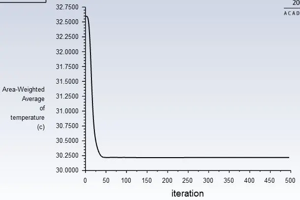
Since the flow through a mixing tee is simulated, it is necessary to simulate the effectiveness mixing at the outlet. This can be done by calculating the average weighted temperature of the fluid at the mixing tee outlet. By doing this we can understand the effect the temperature of hot and cold air, momentum ratio, and the mass flow rate has on the outlet temperature. The area-weighted average temperature at the outlet is approximately 30.25-degrees celsius, and the convergence occurs after the solution has run for approximately 50 iterations.
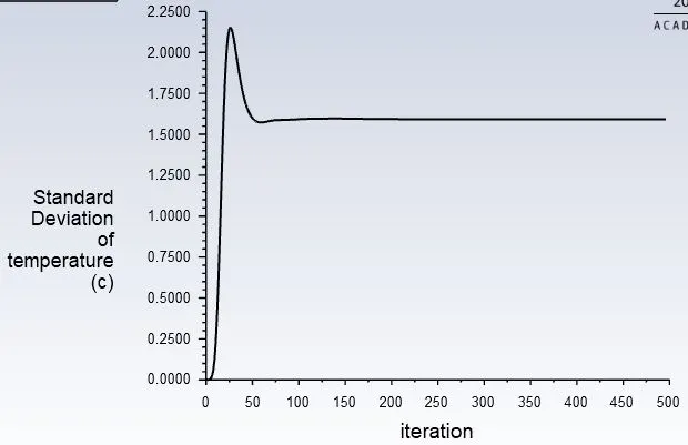
The standard deviation is a statistic that measures the dispersion of a dataset relative to its average. The standard deviation of the temperature at the outlet is approximately 1.6-degrees celsius, and the convergence occurs after the solution has run for approximately 75 iterations.
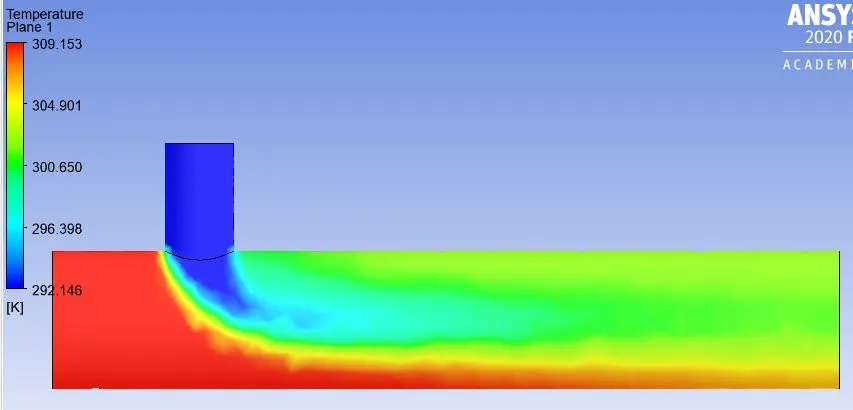
A plane is inserted from the inlet of the pipe to its outlet passing through the center and perpendicular to the inlet-2 cross-section. on this plane, the flow properties temperature and velocity are drawn.
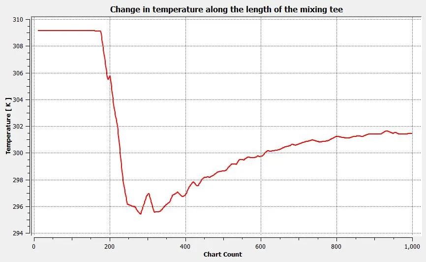
A line is drawn from the inlet of the pipe to its outlet passing through the center, on this line the flow properties temperature and velocity are plotted. The plot above is the temperature profile from the center of the pipe. Initially, the temperature of the air is high, since there is only the flow of hot air. Once the cold air is introduced to the flow, the temperature of the air decreases drastically, and as the flow moves forward, the temperature of flow becomes almost constant due to mixing. The approximate temperature of the fluid near the outlet at the center of the mixing tee is 301.5 0C.
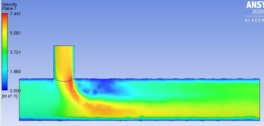
From the above velocity contour plots, we can see the formation of boundary layers near the wall.
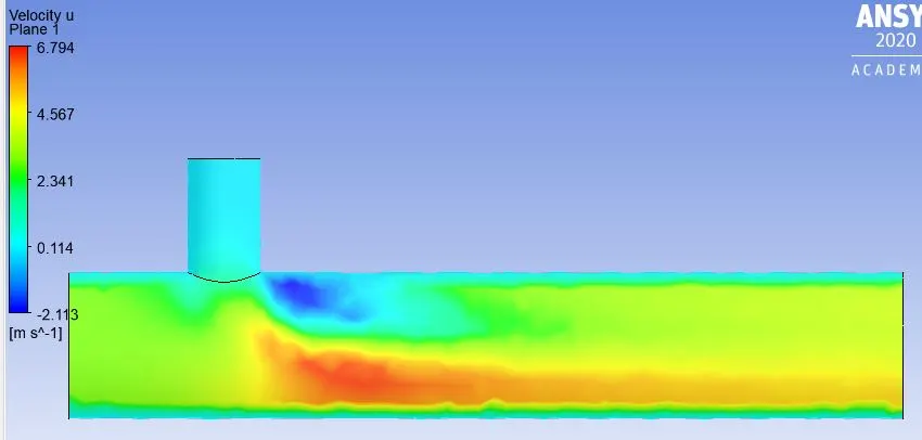
The above contours represent the velocity magnitude along the x-direction. We can see the dark-blue region, wherein the flow velocity is negative. This shows that this region is experiencing reverse flow, The red region represents that the region has the highest magnitude of flow in the x-direction.
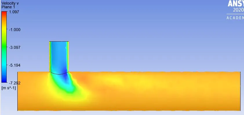
The above contours represent the velocity magnitude along the y-direction. Since the flow from the inlet-2 is in the negative y-direction, the legend shows the velocity as negative.
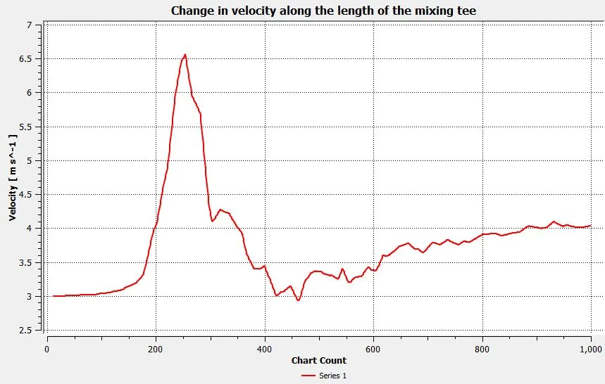
This is the velocity profile from the center of the pipe. Initially, the velocity of the air is 3m/s, since there is only the flow of hot air. Once the cold air with a velocity of 6m/s is introduced to the flow in the negative y-direction, the local velocity of the air increases briefly, and as the flow moves forward, the velocity of flow becomes stabilizes but is greater than the initial velocity at the inlet. The approximate velocity of the fluid at the outlet of the mixing tee is 4m/s.
Mesh independent study:
This study is conducted to check whether or not the mesh size that was used earlier gives accurate results or not. To perform the mesh independence test, the size of the mesh is reduced, without changing the mesh type(tetrahedral mesh in our case). Once this is done, the same simulations are carried out for this case, and a comparison is done between the results obtained using the new mesh and the results obtained using the former mesh. The simulations performed with the finer mesh give more accurate results but they consume a lot of time and resources. Hence if there is no much difference between the results obtained using the new mesh and the former mesh, the former mesh is said to be mesh independent and any further simulations for that particular geometry can be carried out using that mesh.
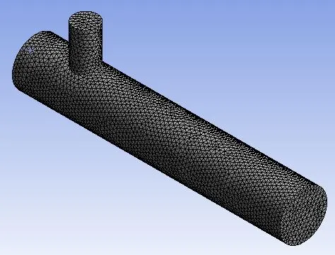
Since we are not interested in the structural analysis of the pipe and we are interested only in the fluid analysis, the volume is extracted from the above geometry, and meshing is done on the fluid by suppressing the solid geometry so that no mesh elements are generated on the pipe. Here tetrahedral meshing is used, with the element size being 0.0025m. This element size is half of the element size used for the earlier simulation. Once the meshing is done there will be a total of 61581 mesh elements for the given geometry.
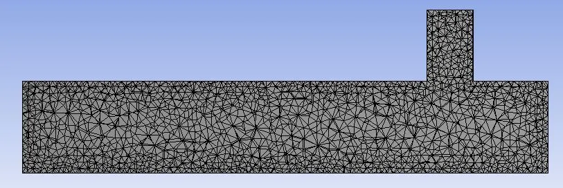
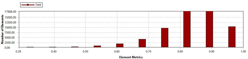
The quality of the mesh is checked, and since the majority of the mesh elements have mesh quality greater than 50%, and there are no mesh elements with mesh quality of less than 25%, the mesh is considered suitable to perform the fluent simulations.
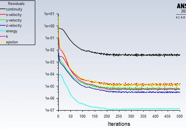
The solver is run for 500 iterations, and from the trend of the residuals plot, we can say that the solution has converged after performing approximately 200 iterations
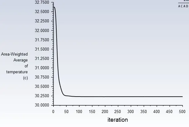
The area-weighted average temperature at the outlet is approximately 30.25-degrees celsius, and the convergence occurs after the solution has run for approximately 50 iterations.
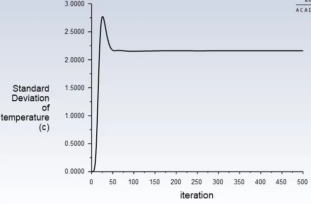
The standard deviation of the temperature at the outlet is approximately 2.2-degrees celsius, and the convergence occurs after the solution has run for approximately 50 iterations.
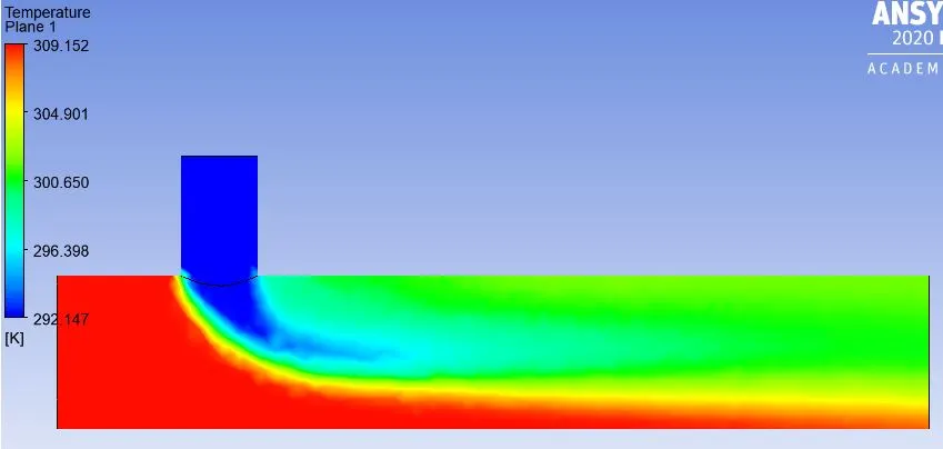
A plane is inserted from the inlet of the pipe to its outlet passing through the center and perpendicular to the inlet-2 cross-section. on this plane, the flow properties temperature and velocity are drawn.
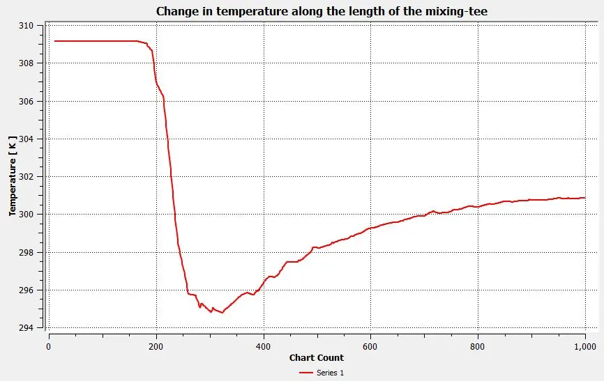
A line is drawn from the inlet of the pipe to its outlet passing through the center, on this line the flow properties temperature and velocity are plotted. The plot above is the temperature profile from the center of the pipe. Initially, the temperature of the air is high, since there is only the flow of hot air. Once the cold air is introduced to the flow, the temperature of the air decreases drastically, and as the flow moves forward, the temperature of flow becomes almost constant due to mixing. The approximate temperature of the fluid near the outlet at the center of mixing tee is 301 0C
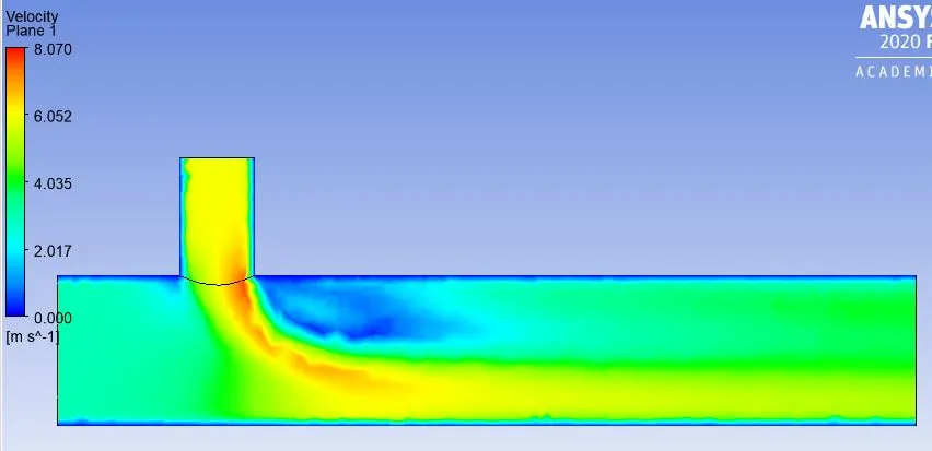
From the above velocity contour plots, we can see the formation of boundary layers near the wall.
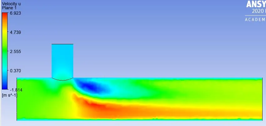
The above contours represent the velocity magnitude along the x-direction. We can see the dark-blue region, wherein the flow velocity is negative. This shows the formation of a vortex during the flow, The red region represents that the region has the highest magnitude of flow in the x-direction.
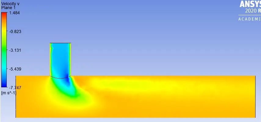
The above contours represent the velocity magnitude along the y-direction. Since the flow from the inlet-2 is in the negative y-direction, the legend shows the velocity as negative.
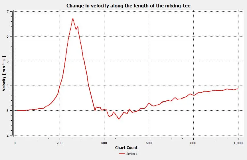
Since the element size is reduced by half, the velocity and temperature contours are can be visualized more clearly. The boundary layer separation, diffusion, flow separation, etc can be seen more clearly. The velocity and temperature line plots and contours which are obtained using the finer mesh are much better compared to the former. The approximate velocity at the outlet of the mixing tee is 3.8m/s.
| Element size | Number of iterations for convergence (appx.) | Average temperature of the fluid after mixing (analytical) (°C) | Area weighted average of temperature at the pipe outlet using Ansys (appx.) (°C) | Standard deviation of temperature at the pipe outlet (appx.) (°C) |
| 0.005 | 200 | 30.33 | 30.25 | 1.6 |
| 0.0025 | 200 | 30.33 | 30.25 | 2.2 |
The above table gives a comparison of results obtained using 2 different element sizes for the mesh. The number of iterations to get a converged solution and the average temperature at the outlet of the mixing tee are the same for both the cases. There is a difference in the standard deviation of temperature values. This is because the finer mesh is able to capture more detail as compared to the coarser mesh. Since the average outlet temperature obtained in both the cases are very close to each other and there is a marginal difference in the value of the standard deviation of temperature at the outlet, the mesh with the mesh element size 0.005m is said to be mesh independent and the remaining simulations are carried out using the same mesh.
1.2) Turbulence model used: K-Omega SST
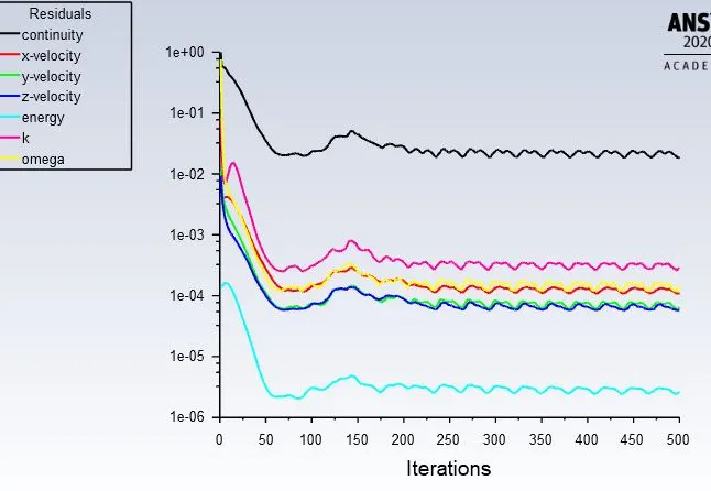
The solver is run for 500 iterations, and from the trend of the residuals plot, we can say that the solution has converged after performing approximately 225 iterations
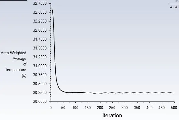
The area-weighted average temperature at the outlet is approximately 30.25-degrees celsius, and the convergence occurs after the solution has run for approximately 75 iterations.
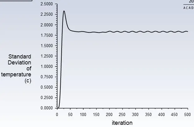
The standard deviation of the temperature at the outlet is approximately 1.75-degrees celsius, and the convergence occurs after the solution has run for approximately 75 iterations.
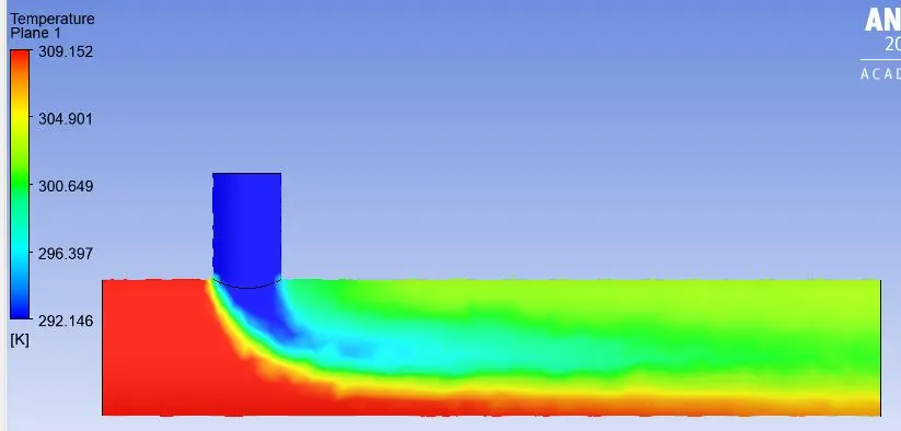
A plane is inserted from the inlet of the pipe to its outlet passing through the center and perpendicular to the inlet-2 cross-section. on this plane, the flow properties temperature and velocity are drawn.
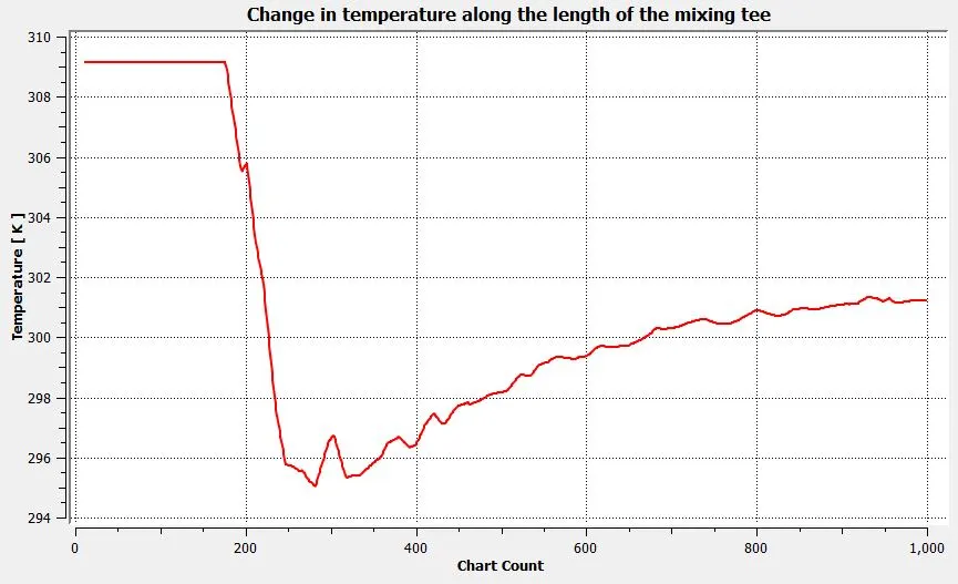
A line is drawn from the inlet of the pipe to its outlet passing through the center, on this line the flow properties temperature and velocity are plotted. The plot above is the temperature profile from the center of the pipe. Initially, the temperature of the air is high, since there is only the flow of hot air. Once the cold air is introduced to the flow, the temperature of the air decreases drastically, and as the flow moves forward, the temperature of flow becomes almost constant due to mixing. The approximate temperature of the fluid near the outlet at the center of mixing tee is 3010C
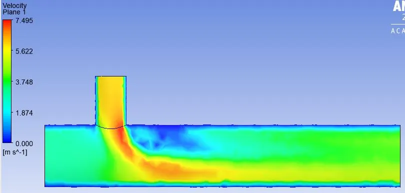
From the above velocity contour plots, we can see the formation of boundary layers near the wall.
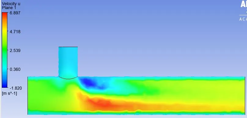
The above contours represent the velocity magnitude along the x-direction. We can see the dark-blue region, wherein the flow velocity is negative. This shows the formation of a vortex during the flow, The red region represents that the region has the highest magnitude of flow in the x-direction.
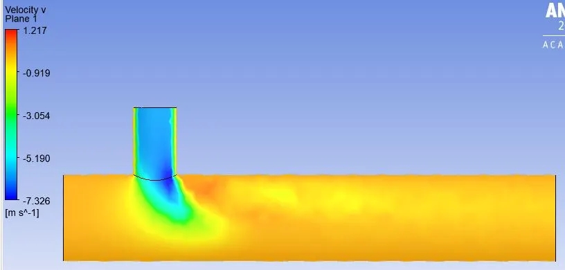
The above contours represent the velocity magnitude along the y-direction. Since the flow from the inlet-2 is in the negative y-direction, the legend shows the velocity as negative.
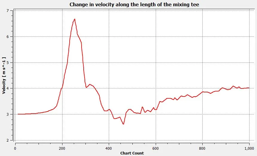
This is the velocity profile from the center of the pipe. Initially, the velocity of the air is 3m/s, since there is only the flow of hot air. Once the cold air with a velocity of 6m/s is introduced to the flow in the negative y-direction, the local velocity of the air increases briefly, and as the flow moves forward, the velocity of flow becomes stabilizes but is greater than the initial velocity at the inlet. The approximate velocity of the fluid at the outlet of the mixing tee is 4m/s.
Comparison between K-epsilon and K-omega SST turbulence models for a momentum ratio of 2:
| Turbulence model used | Number of iterations for convergence (appx.) | Average temperature of the fluid after mixing (analytical) (°C) | Area weighted average of temperature at the pipe outlet using Ansys (appx.) (°C) | Standard deviation of temperature at the pipe outlet (appx.) (°C) |
| K-epsilon | 200 | 30.33 | 30.25 | 1.6 |
| K-omega SST | 225 | 30.33 | 30.25 | 1.75 |
2) momentum ratio =4
For a momentum ratio of 4 and with the velocity of hot air at 3m/s, the velocity of chilled air should be 12m/s. This problem is solved using the K-epsilon and the K-omega SST turbulence model, and comparisons are done between these two models.
2.1) Turbulence model used: K-epsilon
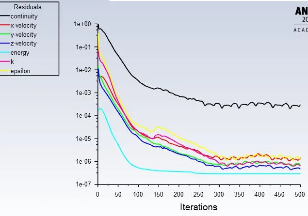
The solver is run for 500 iterations, and from the trend of the residuals plot, we can say that the solution has converged after performing approximately 300 iterations
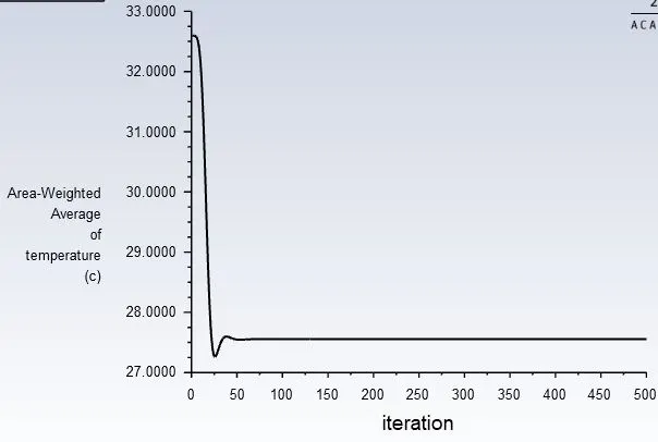
The area-weighted average temperature at the outlet is approximately 27.5-degrees celsius, and the convergence occurs after the solution has run for approximately 50 iterations.
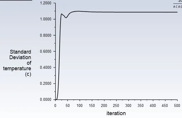
The standard deviation of the temperature at the outlet is approximately 1.1-degrees celsius, and the convergence occurs after the solution has run for approximately 100 iterations.
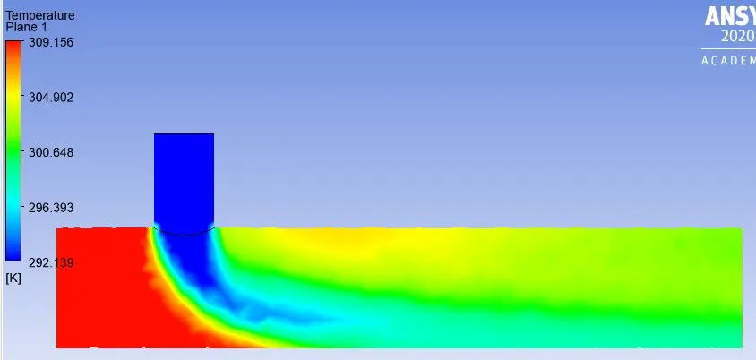
A plane is inserted from the inlet of the pipe to its outlet passing through the center and perpendicular to the inlet-2 cross-section. on this plane, the flow properties temperature and velocity are drawn.
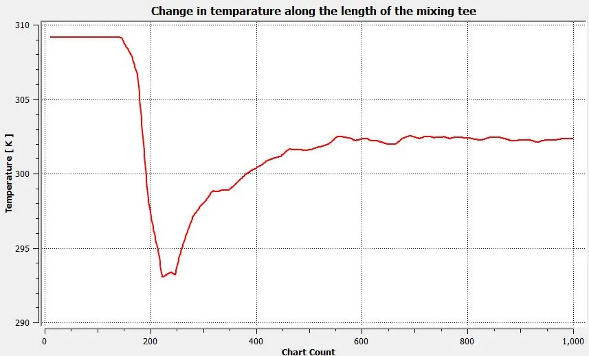
A line is drawn from the inlet of the pipe to its outlet passing through the center, on this line the flow properties temperature and velocity are plotted. The plot above is the temperature profile from the center of the pipe. Initially, the temperature of the air is high, since there is only the flow of hot air. Once the cold air is introduced to the flow, the temperature of the air decreases drastically, and as the flow moves forward, the temperature of flow becomes almost constant due to mixing. The approximate temperature of the fluid near the outlet at the center of the mixing tee is 302 0C.
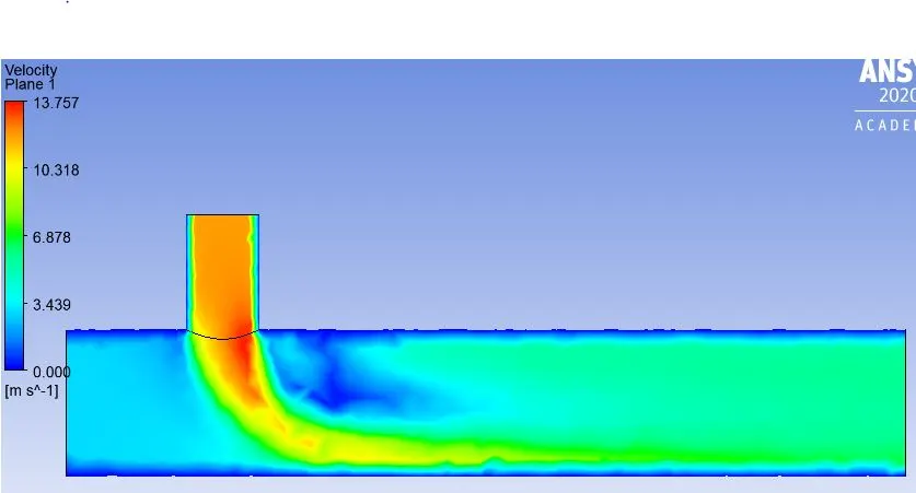
From the above velocity contour plots, we can see the formation of boundary layers near the wall.
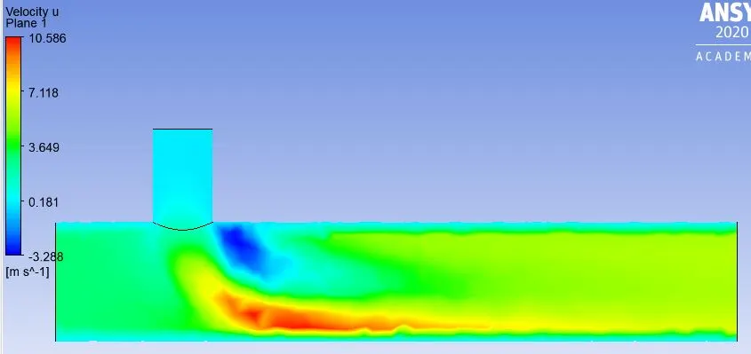
The above contours represent the velocity magnitude along the x-direction. We can see the dark-blue region, wherein the flow velocity is negative. This shows the formation of a vortex during the flow, The red region represents that the region has the highest magnitude of flow in the x-direction.
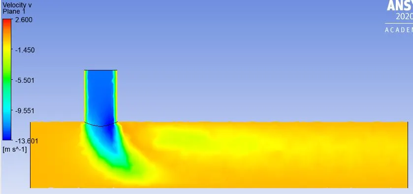
The above contours represent the velocity magnitude along the y-direction. Since the flow from the inlet-2 is in the negative y-direction, the legend shows the velocity as negative.
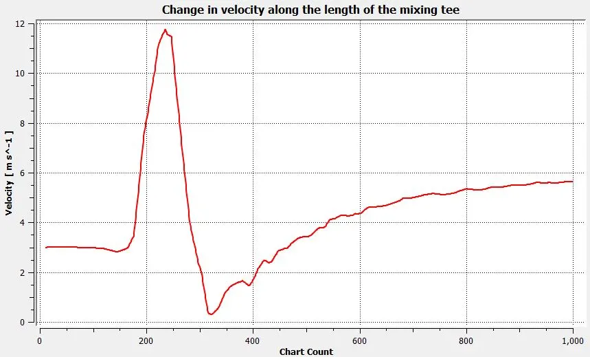
This is the velocity profile from the center of the pipe. Initially, the velocity of the air is 3m/s, since there is only the flow of hot air. Once the cold air with a velocity of 12m/s is introduced to the flow in the negative y-direction, the local velocity of the air increases briefly, and as the flow moves forward, the velocity of flow becomes stabilizes but is greater than the initial velocity at the inlet. The approximate velocity of the fluid at the outlet of the mixing tee is 5.5m/s.
2.2) Turbulence model used: K-omega SST
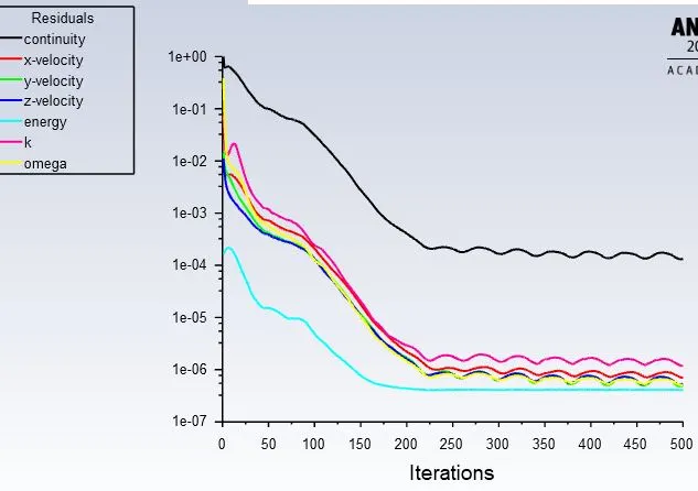
The solver is run for 500 iterations, and from the trend of the residuals plot, we can say that the solution has converged after performing approximately 225 iterations
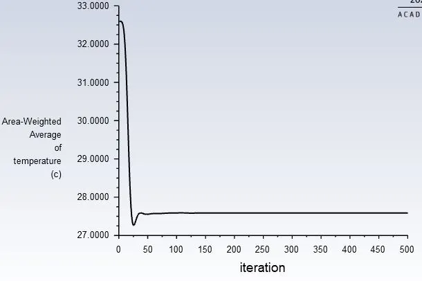
The area-weighted average temperature at the outlet is approximately 27.5-degrees celsius, and the convergence occurs after the solution has run for approximately 50 iterations.
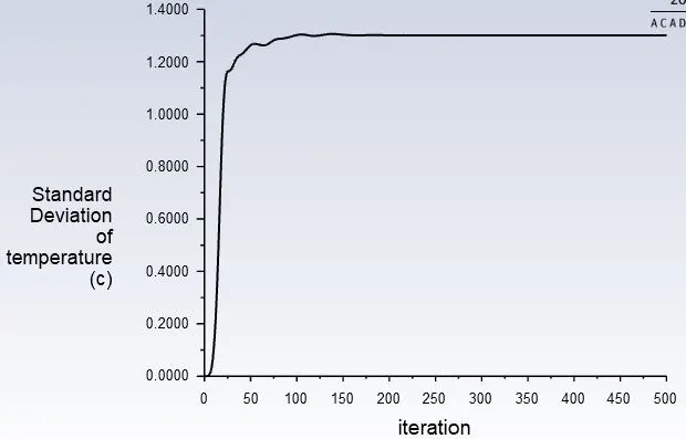
The standard deviation of the temperature at the outlet is approximately 1.3-degrees celsius, and the convergence occurs after the solution has run for approximately 125 iterations.
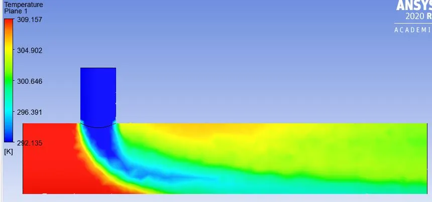
A plane is inserted from the inlet of the pipe to its outlet passing through the center and perpendicular to the inlet-2 cross-section. on this plane, the flow properties temperature and velocity are drawn.
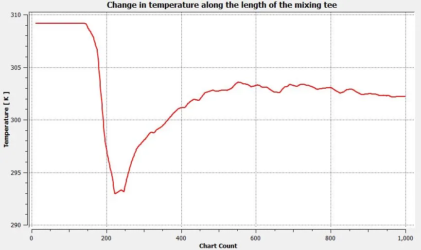
A line is drawn from the inlet of the pipe to its outlet passing through the center, on this line the flow properties temperature and velocity are plotted. The plot above is the temperature profile from the center of the pipe. Initially, the temperature of the air is high, since there is only the flow of hot air. Once the cold air is introduced to the flow, the temperature of the air decreases drastically, and as the flow moves forward, the temperature of flow becomes almost constant due to mixing. The approximate temperature of the fluid near the outlet at the center of mixing tee is 303 0C
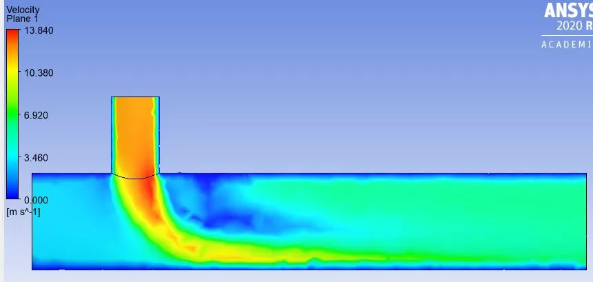
From the above velocity contour plots, we can see the formation of boundary layers near the wall.
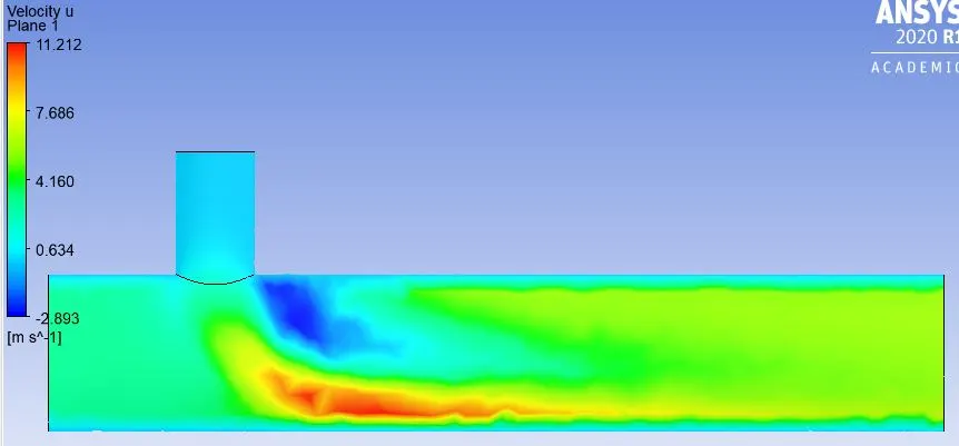
The above contours represent the velocity magnitude along the x-direction. We can see the dark-blue region, wherein the flow velocity is negative. This shows the formation of a vortex during the flow, The red region represents that the region has the highest magnitude of flow in the x-direction.
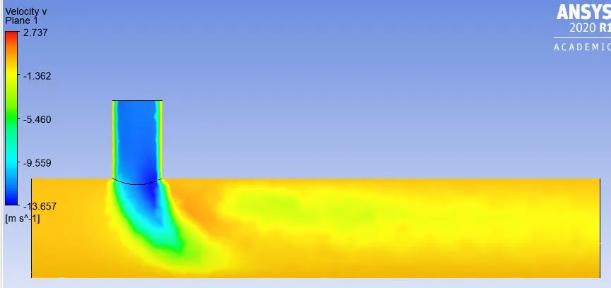
The above contours represent the velocity magnitude along the y-direction. Since the flow from the inlet-2 is in the negative y-direction, the legend shows the velocity as negative.
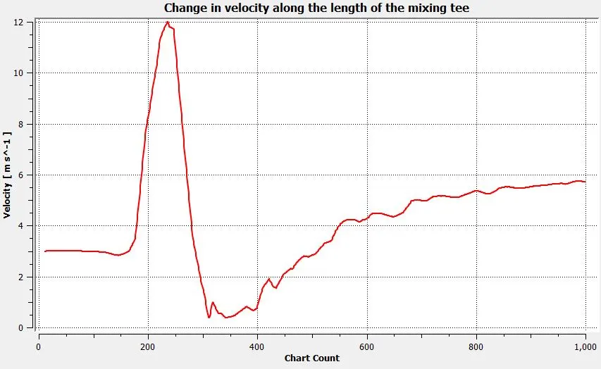
This is the velocity profile from the center of the pipe. Initially, the velocity of the air is 3m/s, since there is only the flow of hot air. Once the cold air with a velocity of 12m/s is introduced to the flow in the negative y-direction, the local velocity of the air increases briefly, and as the flow moves forward, the velocity of flow becomes stabilizes but is greater than the initial velocity at the inlet. The approximate velocity of the fluid at the outlet of the mixing tee is 5.5m/s.
Comparison between K-epsilon and K-omega SST turbulence models for a momentum ratio of 4:
| Turbulence model used | Number of iterations for convergence (appx.) | Average temperature of the fluid after mixing (analytical) (°C) | Area weighted average of temperature at the pipe outlet using Ansys (appx.) (°C) | Standard deviation of temperature at the pipe outlet (appx.) (°C) |
| K-epsilon | 300 | 27.5 | 27.5 | 1.1 |
| K-omega SST | 225 | 27.5 | 27.5 | 1.3 |
Conclusions from running the flow analysis using 2 turbulence models for different momentum ratios:
- The average temperature obtained after complete mixing(ie, at the pipe outlet) using both the turbulence models is almost same and close the solution obtained by hand-calculation
- By increasing the momentum ratio, the temperature of fluid obtained at the outlet is significantly less.
- The standard deviation of temperature at the outlet is higher for the K-omega SST turbulence model compared to the K-epsilon turbulence model for both the momentum ratios. This is because the K-omega SST turbulence model is better for simulating flow near the walls, whereas, the former predicts better far from the wall.
- Since mixing-tee simulation involves wall boundary conditions, the K-omega SST turbulence model is chosen to perform the simulations on further cases.
Case 2: Analysis of long mixing tee using K-omega SST turbulence model
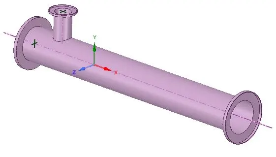
The geometry consists of a pipe with an inner diameter of 34mm, to which another pipe of inner diameter 17mm is attached. The temperature of the air entering the first inlet is of 36-degree celsius, and the temperature of the air entering from the second inlet is 19-degree celsius. The length of the pipe is 268mm.
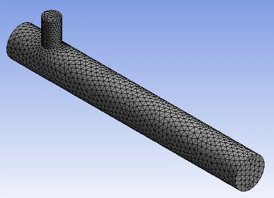
Since we are not interested in the structural analysis of the pipe and we are interested only in the fluid analysis, the volume is extracted from the above geometry, and meshing is done on the fluid by suppressing the solid geometry so that no mesh elements are generated on the pipe. Here tetragonal meshing is used, with the element size being 0.005m. Once the meshing is done there will be a total of 18022 mesh elements for the given geometry.
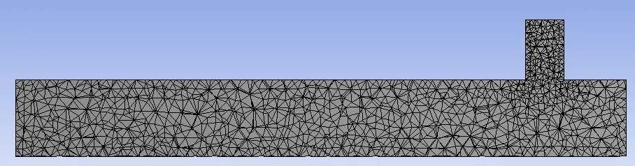
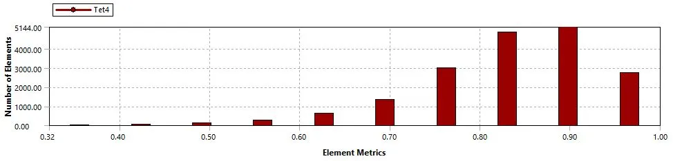
The quality of the mesh is checked, and since the majority of the mesh elements have mesh quality greater than 50%, and there are no mesh elements with mesh quality of less than 30%, the mesh is considered suitable to perform the fluent simulations.
As explained, since we are more interested in the flow near the boundaries, we use the K-omega SST turbulence model to perform the simulation.
1) Momentum ratio =2
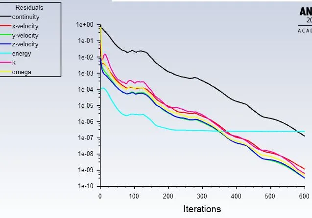
The solver is run for 600 iterations, the trend of the residuals plot shows that the residuals are not stabilizing for given convergence criteria, it is reducing continuously. If we consider the solution to be converged if all the residuals reach the value below 1e-05(convergence criteria), then we can say that the solution has converged after performing approximately 475 iterations.
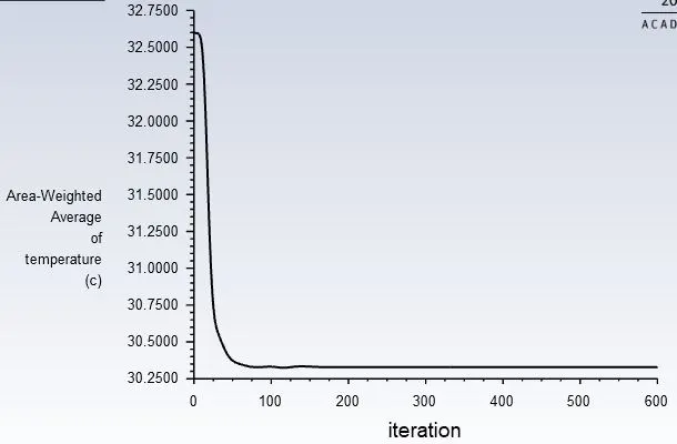
The area-weighted average temperature at the outlet is approximately 30.375-degrees celsius, and the convergence occurs after the solution has run for approximately 75 iterations.
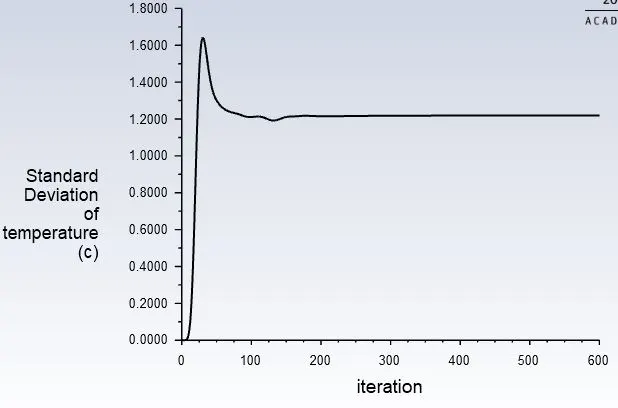
The standard deviation of the temperature at the outlet is approximately 1.2-degrees celsius, and the convergence occurs after the solution has run for approximately 75 iterations.
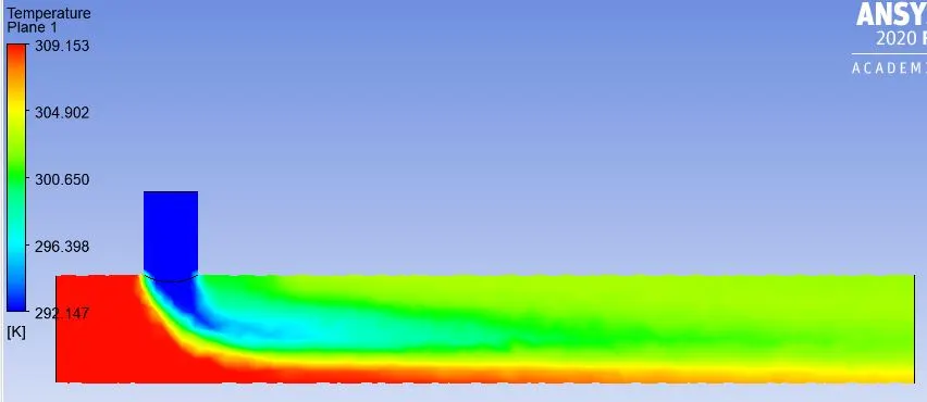
A plane is inserted from the inlet of the pipe to its outlet passing through the center and perpendicular to the inlet-2 cross-section. on this plane, the flow properties temperature and velocity are drawn.
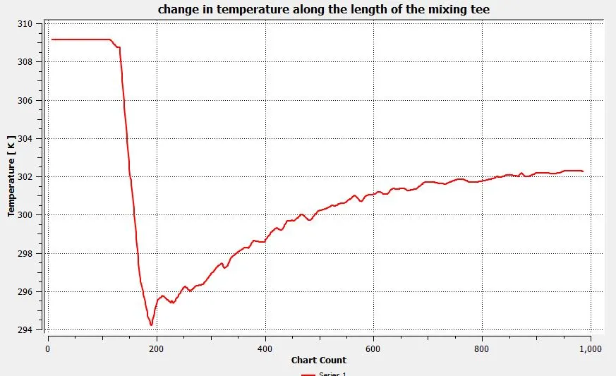
A line is drawn from the inlet of the pipe to its outlet passing through the center, on this line the flow properties temperature and velocity are plotted. The plot above is the temperature profile from the center of the pipe. Initially, the temperature of the air is high, since there is only the flow of hot air. Once the cold air is introduced to the flow, the temperature of the air decreases drastically, and as the flow moves forward, the temperature of flow becomes almost constant due to mixing. The approximate temperature of the fluid near the outlet at the center of mixing tee is 302.5 0C
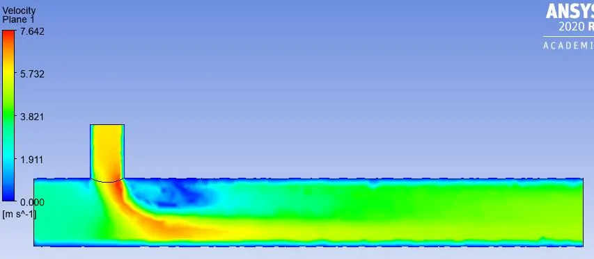
From the above velocity contour plots, we can see the formation of boundary layers near the wall.
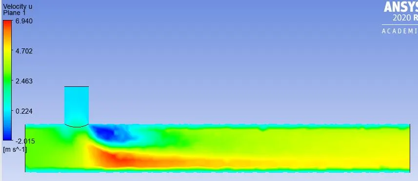
The above contours represent the velocity magnitude along the x-direction. We can see the dark-blue region, wherein the flow velocity is negative. This shows the formation of a vortex during the flow, The red region represents that the region has the highest magnitude of flow in the x-direction.
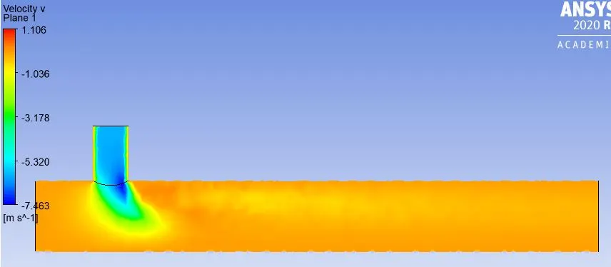
The above contours represent the velocity magnitude along the y-direction. Since the flow from the inlet-2 is in the negative y-direction, the legend shows the velocity as negative.
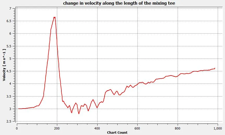
This is the velocity profile from the center of the pipe. Initially, the velocity of the air is 3m/s, since there is only the flow of hot air. Once the cold air with a velocity of 6m/s is introduced to the flow in the negative y-direction, the local velocity of the air increases briefly, and as the flow moves forward, the velocity of flow becomes stabilizes but is greater than the initial velocity at the inlet. The approximate velocity of the fluid at the outlet of the mixing tee is 4.2m/s.
2) Momentum ratio =4
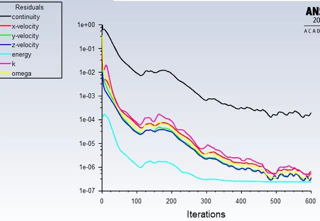
The solver is run for 600 iterations, and from the trend of the residuals plot, we can say that the solution has converged after performing approximately 450 iterations
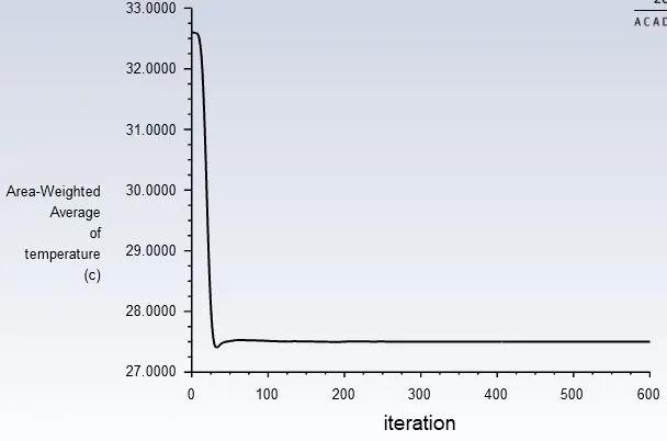
The area-weighted average temperature at the outlet is approximately 27.5-degrees celsius, and the convergence occurs after the solution has run for approximately 50 iterations.
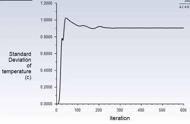
The standard deviation of the temperature at the outlet is approximately 0.9-degrees celsius, and the convergence occurs after the solution has run for approximately 100 iterations.
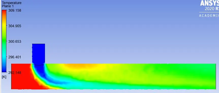
A plane is inserted from the inlet of the pipe to its outlet passing through the center and perpendicular to the inlet-2 cross-section. on this plane, the flow properties temperature and velocity are drawn.
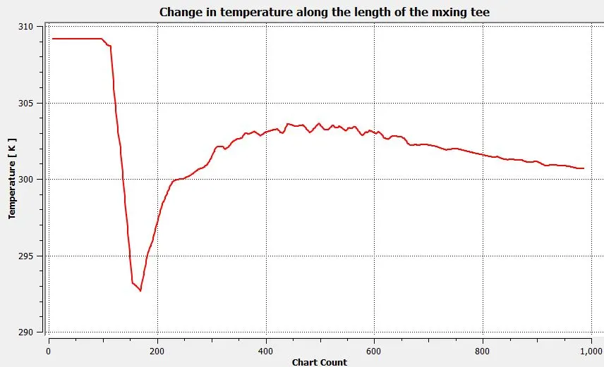
A line is drawn from the inlet of the pipe to its outlet passing through the center, on this line the flow properties temperature and velocity are plotted. The plot above is the temperature profile from the center of the pipe. Initially, the temperature of the air is high, since there is only the flow of hot air. Once the cold air is introduced to the flow, the temperature of the air decreases drastically, and as the flow moves forward, the temperature of flow becomes almost constant due to mixing. The approximate temperature of the fluid near the outlet at the center of mixing tee is 301 0C
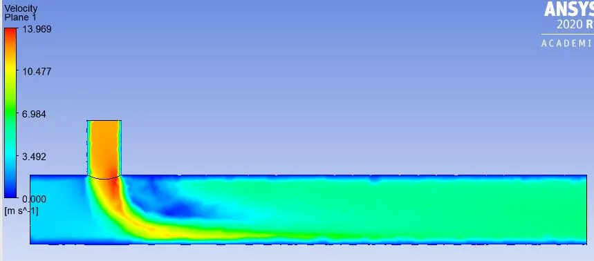
From the above velocity contour plots, we can see the formation of boundary layers near the wall.
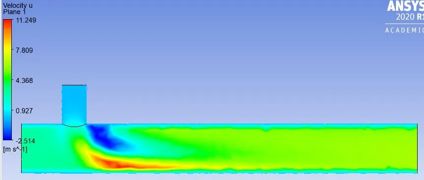
The above contours represent the velocity magnitude along the x-direction. We can see the dark-blue region, wherein the flow velocity is negative. This shows the formation of a vortex during the flow, The red region represents that the region has the highest magnitude of flow in the x-direction.
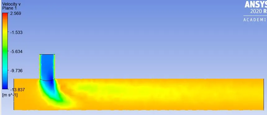
The above contours represent the velocity magnitude along the y-direction. Since the flow from the inlet-2 is in the negative y-direction, the legend shows the velocity as negative.
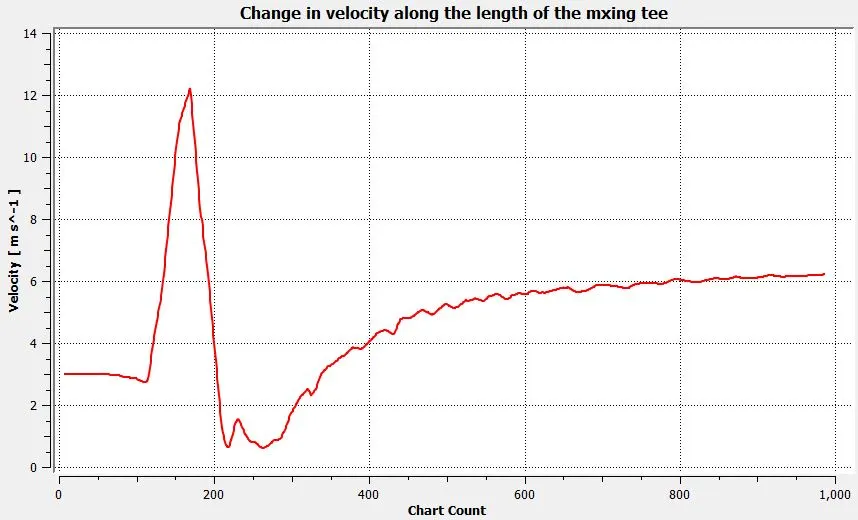
This is the velocity profile from the center of the pipe. Initially, the velocity of the air is 3m/s, since there is only the flow of hot air. Once the cold air with a velocity of 12m/s is introduced to the flow in the negative y-direction, the local velocity of the air increases briefly, and as the flow moves forward, the velocity of flow becomes stabilizes but is greater than the initial velocity at the inlet. The approximate velocity of the fluid at the outlet of the mixing tee is 6.5m/s.
Comparison of the results obtained for different momentum ratios:
| Momentum ratio | Number of iterations for convergence (appx.) | Average temperature of the fluid after mixing (analytical) (°C) | Area weighted average of temperature at the pipe outlet using Ansys (appx.) (°C) | Standard deviation of temperature at the pipe outlet (appx.) (°C) |
| 2 | 475 | 30.33 | 30.375 | 1.2 |
| 4 | 450 | 27.5 | 27.5 | 0.9 |
Final results:
| Length of the mixing-tee | Cell count | Turbulence model used | momentum ratio | Number of iterations for convergence (appx.) | Average outlet temperature | Standard deviation of temperature at the outlet |
| Short(192mm) | 14197 | K-epsilon | 2 | 200 | 30.25 | 1.6 |
| K-omega SST | 225 | 30.25 | 1.75 | |||
| K-epsilon | 4 | 300 | 27.5 | 1.1 | ||
| K-omega SST | 225 | 27.5 | 1.3 | |||
| Long(278mm) | 18022 | K-omega SST | 2 | 475 | 30.375 | 1.2 |
| 4 | 450 | 27.5 | 0.9 |
Conclusions:
- The mesh element size of 0.005m is proved to be mesh independent, ie, any simulation can be run using that mesh to get accurate results, and even if the mesh is further refined, there will be a minimal effect on the accuracy of the solution.
- Increasing the momentum ratio significantly reduces the average temperature of the air at the mixing tee outlet.
- Increasing the length of the pipe has minimal effect on the outlet temperature. If the length of the pipe is increased, the air gets mixed evenly, hence there is a decrease in the value of the standard deviation of temperature for long mixing tee compared to short mixing tee for the same momentum ratio. Increasing the length of the pipe has no effect on reducing the outlet temperature.
- The K-epsilon turbulence model is more accurate in predicting the results far from the wall, whereas the K-omega SST is better at predicting the results near the wall. Due to this property, the standard deviation of temperature found using the K-omega SST turbulence model is marginally higher compared to that of the K-epsilon turbulence model. This is the reason for choosing the K-omega SST turbulence model instead of the K-epsilon turbulence model to perform simulation for case 2.