Solving the steady and unsteady 2D heat conduction equations.

Aim:

To perform steady-state analysis & transient state analysis to solve the 2D heat conduction equation by using the point iterative techniques by implementing the following methods:

1. Jacobi method

2. Gauss-seidel method

3. Successive over-relaxation (SOR) method

absolute error criteria = 1e-4

Assumptions:

• The analysis will be done on a square plate, with an equal number of grid points on x and y axes (nx=ny). Therefore `Deltax=Deltay``
• Thermal diffusivity(`omega`) is taken as 2.5
• There is no heat generated on the matrix, ie, the heat generation term is zero
• The length of the domain is (1*1)m
• The temperatures at left, top, right, and bottom wall are 400K, 600K, 800K, 900K respectively
• The temperatures at the corner grid are taken as the athematic average of its corresponding walls
• The solution is said to be converged if the absolute error term in each and every grid at least becomes less than 1e-4 while performing the iterations.

Case1: Steady-state analysis

The generalized 2D temperature equation for the steady-state condition is,

`(∂^2T)/(∂x^2)+(∂^2T)/(∂y^2)=0`

When we discretize the equation by the central differencing scheme, we get,

`(T_(i−1,j)−2T_(i,j)+T_(i+1,j))/(Deltax^2)+(T_(i,j-1)−2T_(i,j)+T_(i,j+1))/(Deltay^2)=0`

since `Deltax=Deltay`, the equation reduces to

`T_(i,j)=(1/4)*(T_(i−1,j)+T_(i+1,j)+T_(i,j−1)+T_(i,j+1))`---(1)`

The heat conduction equation can be solved by the following methods:

1) Jacobi method: Here the value of temperature taken will be the same as that of the previous iteration.

In equation (1), the value of terms T(i-1,j) and T(I,j-1) are computed in the current iteration, but while solving the equation by using the Jacobi method, the temperature values computed in the previous iteration is substituted

2) Gauss-Seidel method: Here the value of temperature substituted will be the latest value computed.

In equation (1), the value of terms T(i-1,j) and T(I,j-1) are computed in the current iteration, these updated values are then substituted in the equation rather than the values obtained in the previous iteration

3) Successive over-relaxation method (SOR): In this method, the scaling factor is introduced in addition to the Jacobi or Gauss-Seidel method which is used within this method. The scaling factor reduces the number of iterations required in obtaining converged results and subsequently reducing computing time.

The final equation will be: `(1-omega)T_(old)+omega(T_J or T_(GS))`

If omega> 1, then it is over-relaxed

If omega<1, then it is under relaxed.

Matlab/Octave code:

close all
clear all
clc

% Inputs
L =  1;
nx = 20;
ny = nx;
x = linspace(0,L,nx);
y = linspace(0,L,ny);
dx = x(2)-x(1);
dy = y(2)-y(1);
error = 9e9;
tol = 1e-4;

% Defining boundary conditions
% Temperature at boundaries
T_L = 400;
T_T = 600;
T_R = 800;
T_B = 900;
T = 675*ones(nx,ny);

T(2:ny-1,1) = T_L;
T(2:ny-1,nx) = T_R;
T(1,2:nx-1) = T_B;
T(nx,2:ny-1) = T_T;

% calculating average temperature at the corners
T(1,1) = (T_B + T_L)/2;
T(nx,ny) = (T_R + T_T)/2;
T(ny,1) = (T_T + T_L)/2;
T(1,nx) = (T_R + T_B)/2;

% for 2D representation
[X,Y] = meshgrid(x,y);

% making a copy
Told = T;

% Calculation of 2d Steady state heat conduction eqn 
iterative_solver=3;

% Jacobi method

if iterative_solver==1
% to find computation time
tic; 
if iterative_solver==1
    jacobi_iter=1;
    while(error > tol)
        for i=2:nx-1
            for j=2:ny-1
                T(i,j) = 0.25*((Told(i-1,j)+Told(i+1,j)+Told(i,j-1)+Told(i,j+1)));
            end
        end
        error = max(max(abs(Told-T)));
        Told = T;
        jacobi_iter=jacobi_iter+1;  
    end
end
% to end computing time 
F=toc;

%plot
figure(1)
[M,N]=contourf(X,Y,T);
clabel(M,N)
colormap(jet)
colorbar
title_text=sprintf('Number of iterations using Jacobi method=%d, Computation time=%fs',jacobi_iter,F);
title(title_text)
xlabel('X-axis')
ylabel('Y-axis')
fprintf('Number of Iterations using Jacobi method=%dn',jacobi_iter);
end

% Gauss/Seidel method

if iterative_solver==2
% to find computation time
tic; 
if iterative_solver==2
    gs_iter=1;
    while(error > tol)
        for i=2:nx-1
            for j=2:ny-1
                T(i,j) = 0.25*((T(i-1,j)+Told(i+1,j)+T(i,j-1)+Told(i,j+1)));
            end
        end
        error = max(max(abs(Told-T)));
        Told = T;
        gs_iter=gs_iter+1;  
    end
end
% to end computing time 
F=toc;

%plot
figure(2)
[M,N]=contourf(X,Y,T);
clabel(M,N)
colormap(jet)
colorbar
title_text=sprintf('Number of iterations using G-S method=%d, Computation time=%fs',gs_iter,F);
title(title_text)
xlabel('X-axis')
ylabel('Y-axis')
fprintf('Number of Iterations using G-S method=%dn',gs_iter);
end

a = 1.72

% SOR method using G-S equation

if iterative_solver==3
% to find computation time
tic; 
if iterative_solver==3
    SOR_iter=1;
    while(error > tol)
        for i=2:nx-1
            for j=2:ny-1
                T(i,j) = ((1-a)*Told(i,j)+(a*0.25*(T(i,j-1)+Told(i,j+1)+T(i-1,j)+Told(i+1,j))));
            end
        end
        error = max(max(abs(Told-T)));
        Told = T;
        SOR_iter=SOR_iter+1;  
    end
end
% to end computing time 
F=toc;

%plot
figure(3)
[M,N]=contourf(X,Y,T);
clabel(M,N)
colormap(jet)
colorbar
title_text=sprintf('Number of iterations using G-S formula in SOR method=%d, Computation time=%fs',SOR_iter,F);
title(title_text)
xlabel('X-axis')
ylabel('Y-axis')
fprintf('Number of iterations using GS formula in SOR method=%dn',SOR_iter);
end

Outputs:

a) Jacobi method

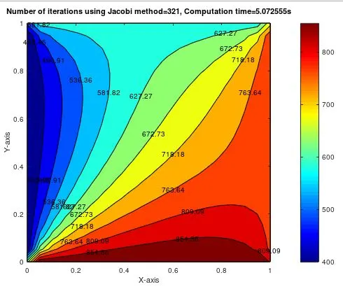
when the equation was solved using the Jacobi formula, It took 321 iterations to get converged results. The time taken to perform the iterations is approximately 5s.

b) Gauss-Seidel method

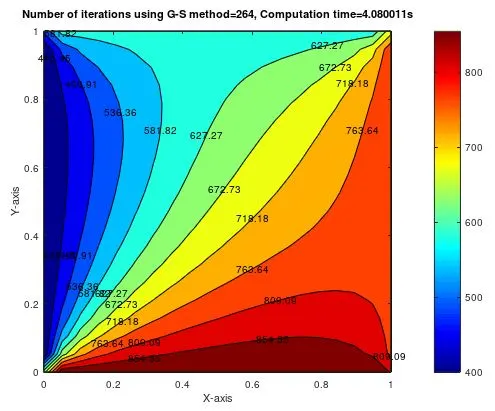
When the equation was solved using the Gauss-Seidel formula, It took 264 iterations to get converged results. This is much lower compared to the number of iterations taken to solve the same equation using the Jacobi method. Due to this the time required for computation reduces significantly compared to that of the Jacobi method. This is because the terms substituted in the discretized equation are the latest terms computed, rather than substituting the terms obtained in the previous iteration.

c) Successive over-relaxation method (SOR)

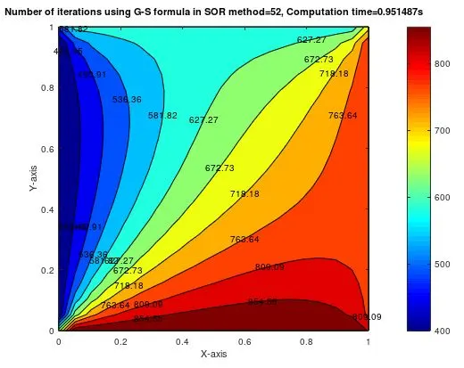
When the equation was solved using the successive over-relaxation method using the Gauss-Seidel formula, it took just 52 iterations to get converged results. Since the result was obtained with a lesser number of iterations, the computation time reduced significantly, in our case it is approximately 0.95s. Here the scaling factor, omega was taken as 1.72. This value of omega was found by trial and error method. First, the value of omega was given 1.1 and then increased continuously by 0.1. The number of iterations kept reducing up to 1.7 but increased at 1.8. Once this upper-limit was obtained, the value of omega was increased continuously by 0.01 from 1.7. The lowest number of iterations was found to be at omega=1.72, so this value was chosen as the scaling factor for solving this problem.

The main reason for the introduction of this method is for the faster convergence of results. From the first two methods, it was clear that the Gauss-Seidel method is more efficient than the Jacobi method. This is the reason why the Gauss-Seidel formula was used in the successive over-relaxation method instead of the former.

Case2: Transient/unsteady state analysis

The generalized 2D conduction equation for unsteady/transient case is given by,

`(delT)/(delt)=alpha((del^2T)/(delx^2)+(del^2T)/(dely^2))`---(2)

This equation can be solved implicitly or explicitly

case2a: Transient/unsteady state analysis using the explicit method

discretizing equation (2) using the central difference scheme, we get,

`(T_p^(n+1)-T_p^n)/(Deltat)=alpha((T_L-2T_P+T_R)/(Deltax^2)+(T_T-2T_P+T_B)/(Deltay^2))^n`

If the problem is solved at time step n, then it is called the explicit method. If the problem is solved at time step n+1, then it is called implicit method.

Simplifying the equation for explicit method, we get,

`T_P^(n+1)=T_P^n+K1(T_L-2T_P+T_R)^n+K2(T_T-2T_P+T_B)^n`

Where `K1=alpha(Deltat)/(Deltax^2) and K2=alpha(Deltat)/(Deltay^2)`

For easier substitution of the formula in the code, the following terms are defined:

`Term1 = T_P^n`

`Term2 = K1*(T_L-2*T_P+T_R)^n`

`Term3 = K2*(T_T-2T_P+T_B)^n`

The final equation:

`T_P^(n+1)= Term1+Term2+Term3`

Matlab/Octave code:

close all
clear all
clc

% Inputs
L = 1;

% no of grid points along X & Y
nx = 11;
ny = nx;
x = linspace(0,L,nx);
y = linspace(0,L,ny);

dx = x(2)-x(1);
dy = y(2)-y(1);

error = 9e9;
tol = 1e-4;
dt = 0.001; % time step
alpha = 2.5; % thermal diffusivity

% Defining boundary conditions
T_L = 400;
T_T = 600;
T_R = 800;
T_B = 900;

% Initial condition
T = 675*ones(nx,ny);

T(2:ny-1,1) = T_L;
T(2:ny-1,nx) = T_R;
T(1,2:nx-1) = T_B;
T(nx,2:ny-1) = T_T;

% calculating average temperature at the matrix corners
T(1,1) = (T_B + T_L)/2;
T(nx,ny) = (T_R + T_T)/2;
T(ny,1) = (T_T + T_L)/2;
T(1,nx) = (T_R + T_B)/2;

% other factors to be considered
% we know the values for constants k1 and k2

k1 = (alpha*dt)/(dx^2);
k2 = (alpha*dt)/(dy^2);

% for 2D representation
[X,Y] = meshgrid(x,y);

% making a copy
Told = T;

% Calculation of 2d Transient state heat conduction eqn in Explicit

iterative_solver=1;
% To calculate computation time
tic; 
if iterative_solver==1
  count=1
    while(error > tol)
        for i=2:nx-1
            for j=2:ny-1
                term1 = Told(i,j);
                term2 = k1*(Told(i+1,j)-2*Told(i,j)+Told(i-1,j));
                term3 = k2*(Told(i,j+1)-2*Told(i,j)+Told(i,j-1));
                T(i,j)= term1+term2+term3 
            end
        end
        error = max(max(abs(Told-T)));
        Told = T;
        count = count+1;  
    end
end
% To end computing time
F=toc;

%% plot
figure(1)
[M,N]=contourf(X,Y,T);
clabel(M,N)
colormap(jet)
colorbar
title_text=sprintf('Number of iterations performed =%d, Computation Time=%fs',count,F);
title(title_text)
xlabel('X-axis')
ylabel('Y-axis')
fprintf('Number of iterations performed to solve unsteady-state conduction problem using explicit method=%dn',count);

Output:

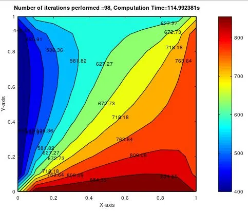
This code was run on Octave. The thermal diffusivity term was taken as 2.5, and the time step dt=0.001. The number of grid points in both x and y direction is taken as 11. The initial temperature at all grid points is taken as the average temperature of the four walls. These values are taken for the faster convergence of the solution, else the solution will take a lot of time to converge. These values were chosen carefully, such that the sum of terms K1 and K2 does not exceed 0.5, else the solution will become unstable. When the code was run for the said initial and boundary conditions, the solution gets converged after 98 iterations, and the time taken to perform the iterations is approximately 115s.

case2b: Transient/unsteady state analysis using the implicit method

discretizing equation (2) using the central difference scheme, we get,

`(T_p^(n+1)-T_p^n)/(Deltat)=alpha((T_L-2T_P+T_R)/(Deltax^2)+(T_T-2T_P+T_B)/(Deltay^2))^(n+1)`

Simplifying the equation for implicit method, we get,

`T_P^(n+1)=(1/(1+2K1+2K2))(T_P^n+K1(T_L+T_R)^(n+1)+K2(T_T+T_B)^(n+1))`

where `K1=alpha(Deltat)/(Deltax^2) and K2=alpha(Deltat)/(Deltay^2)`

For easier substitution of the formula in the code, the following terms are defined:

`Term1=1/(1+2K_1+2K_2)`

`Term2=K_1*Term1`

`Term2=K_2*Term1`

Matlab/Octave code:

close all
clear all
clc

% Inputs
L =  1;
nx = 11;
ny = nx;
x = linspace(0,L,nx);
y = linspace(0,L,ny);

dx = x(2)-x(1);
dy = y(2)-y(1);

error = 9e9;
tol = 1e-4;
dt = 0.001; % time step
alpha = 2.5; % thermal diffusivity

% other factors to be considered
% we know the values for constants k1 and k2

k1 = (alpha*dt)/(dx^2);
k2 = (alpha*dt)/(dy^2);

% Defining boundary conditions
% Temperature at boundaries
T_L = 400;
T_T = 600;
T_R = 800;
T_B = 900;
T = 675*ones(nx,ny);

T(2:ny-1,1) = T_L;
T(2:ny-1,nx) = T_R;
T(1,2:nx-1) = T_B;
T(nx,2:ny-1) = T_T;

% calculating average temperature at the corners
T(1,1) = (T_B + T_L)/2;
T(nx,ny) = (T_R + T_T)/2;
T(ny,1) = (T_T + T_L)/2;
T(1,nx) = (T_R + T_B)/2;



% for 2D representation
[X,Y] = meshgrid(x,y);

% making a copy
Told = T;
Tprev = T;

Term1 = (1+(2*k1)+(2*k2))^(-1);
Term2 = k1*Term1;
Term3 = k2*Term1;

% Calculation of 2D transient state heat conduction eqn 
iterative_solver=3;

% Jacobi method

if iterative_solver==1
% to find computation time
tic; 
if iterative_solver==1
    jacobi_iter=1;
    for nt=1:1500
    error = 1;
    while(error > tol)
        for i=2:nx-1
            for j=2:ny-1
                H = Told(i-1,j)+Told(i+1,j);
                V = Told(i,j-1)+Told(i,j+1);
                T(i,j) = (Tprev(i,j)*Term1)+(H*Term2)+(V*Term3);
            end
        end
        error = max(max(abs(Told-T)));
        Told = T;
        jacobi_iter=jacobi_iter+1;  
    end
    Tprev = T;
    end
end

% to end computing time 
F=toc;

%plot
figure(1)
[M,N]=contourf(X,Y,T);
clabel(M,N)
colormap(jet)
colorbar
title_text=sprintf('Number of iterations using Jacobi method=%d, Computation time=%fs',jacobi_iter,F);
title(title_text)
xlabel('X-axis')
ylabel('Y-axis')
fprintf('Number of Iterations using Jacobi method=%dn',jacobi_iter);
end

% Gauss/Seidel method

if iterative_solver==2
% to find computation time
tic; 
if iterative_solver==2
    gs_iter=1;
    for nt=1:1500
    error=1;
    while(error > tol)
        for i=2:nx-1
            for j=2:ny-1
                H = T(i-1,j)+Told(i+1,j);
                V = T(i,j-1)+Told(i,j+1);
                T(i,j) = (Tprev(i,j)*Term1)+(H*Term2)+(V*Term3);
            end
        end
        error = max(max(abs(Told-T)));
        Told = T;
        gs_iter=gs_iter+1;  
    end
    Tprev = T;
    end
end
% to end computing time 
F=toc;

%plot
figure(2)
[M,N]=contourf(X,Y,T);
clabel(M,N)
colormap(jet)
colorbar
title_text=sprintf('Number of iterations using G-S method=%d, Computation time=%fs',gs_iter,F);
title(title_text)
xlabel('X-axis')
ylabel('Y-axis')
fprintf('Number of Iterations using G-S method=%dn',gs_iter);
end

a = 1.2

% SOR method using G-S equation

if iterative_solver==3
% to find computation time
tic; 
if iterative_solver==3
    SOR_iter=1;
    for nt=1:1500
    error=1;
    while(error > tol)
        for i=2:nx-1
            for j=2:ny-1
                H = T(i-1,j)+Told(i+1,j);
                V = T(i,j-1)+Told(i,j+1);
                T(i,j) = (Told(i,j)*(1-a))+a*((Tprev(i,j)*Term1)+(H*Term2)+(V*Term3));
            end
        end
        error = max(max(abs(Told-T)));
        Told = T;
        SOR_iter=SOR_iter+1;  
    end
    Tprev = T;
    end
end
% to end computing time 
F=toc;

%plot
figure(3)
[M,N]=contourf(X,Y,T);
clabel(M,N)
colormap(jet)
colorbar
title_text=sprintf('Number of iterations using G-S formula in SOR method=%d, Computation time=%fs',SOR_iter,F);
title(title_text)
xlabel('X-axis')
ylabel('Y-axis')
fprintf('Number of iterations using GS formula in SOR method=%dn',SOR_iter);
end

Outputs:

a) Jacobi method

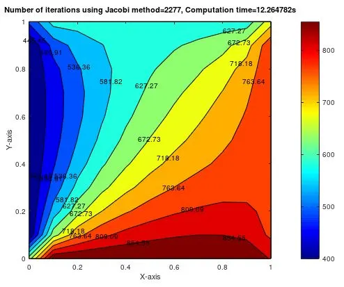
When the transient state heat conduction problem is solved using the Jacobi method with the given initial conditions, the solution gets converged after 2277 iterations. The time taken to perform these iterations is about 12s.

b) Gauss-Seidel method

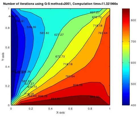
When the equation was solved using the Gauss-Seidel formula, It took 2051 iterations to get converged results. This is much lower compared to the number of iterations taken to solve the same equation using the Jacobi method. Due to this the time required for computation reduces significantly compared to that of the Jacobi method. This is because the terms substituted in the discretized equation are the latest terms computed, rather than substituting the terms obtained in the previous iteration.

c) Successive over-relaxation method

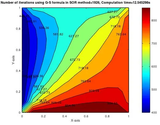
When the equation was solved using the successive over-relaxation method using the Gauss-Seidel formula, it took just 1926 iterations to get converged results. Here the scaling factor, omega was taken as 1.2. This value of omega was found by trial and error method. First, the value of omega was given 1.1 and then increased continuously by 0.1. The number of iterations kept reducing up to 1.2 but increased at 1.3. So to the value of omega was taken as 1.3.

The main reason for the introduction of this method is for the faster convergence of results. From the first two methods, it was clear that the Gauss-Seidel method is more efficient than the Jacobi method. This is the reason why the Gauss-Seidel formula was used in the successive over-relaxation method instead of the former. Though in our we get the computation time in case of SOR slightly more than that of the Gauss-Seidel method, the number of iterations are comparatively less.

Results:

a) Steady-state 2D heat conduction

This equation is solved using three methods namely Jacobi, Gauss-Seidel, and Successive over-relaxation method and the following results obtained:

Method used	Number of iterations	Time taken to perform the iterations (s)
Jacobi method	321	5.072555
Gauss-Seidel method	264	4.080011
Successive over-relaxation method	52	0.951487

b) Transient-state 2D heat conduction (explicit)

The transient-state is solved explicitly and the solution gets converged after 98 iterations, and the time taken to perform the iterations is 114.992381s.

c) Transient-state 2D heat conduction (implicit)

This equation is solved using three methods namely Jacobi, Gauss-Seidel, and Successive over-relaxation method and the following results obtained:

Method used	Number of iterations	Time taken to perform the iterations (s)
Jacobi method	2277	12.264782
Gauss-Seidel method	2051	11.321966
Successive over-relaxation method	1926	12.545298

Conclusions:

1. Steady-state conduction is the form of conduction that happens when the temperature difference driving the conduction is constant with respect to time. On the other hand, in transient-state condition, the temperature at the boundaries changes with time, and eventually reach a steady state if the temperature is not changed further.
2. If the error term obtained is below the tolerance value, the solution is said to be converged. In the above problem which is solved in steady and unsteady-state conditions, we obtain an error term below the tolerance value(1e-4) for each case, hence the solution is converged.
3. In the steady-state analysis and transient-state analysis using the implicit method, the solution is obtained using three methods, namely, Jacobi(J), Gauss-Seidel(GS), and successive over-relaxation(SOR) method. Out of these three methods, the third method, SOR converges to the solution with a lower number of iterations compared to the other two methods, provided that the value of omega is appropriate. The Jacobi method in both cases converges to the solution with the highest number of iterations compared to the other two methods.
4. From this, we can conclude that the successive over-relaxation method is the most effective method since it converges the solution for a lesser number of iterations and hence less time is taken for solving compared to Jacobi and Gauss-Seidel method. This largely depends on the value of omega, if an appropriate value is chosen, then the solution converges faster, else the solution may take longer to converge.