Simulation of Rayleigh-Taylor instability

Aim:

To perform Rayleigh Taylor instability simulation on a 2D multiphase setup.

Problem statements:

1. To perform the Rayleigh Taylor instability simulation with water and air for 2 different mesh sizes with the base mesh being 0.5 mm.
2. To perform the Rayleigh Taylor instability simulation with water and user-defined material (density= 400kg/m^3, viscosity= 0.001kg/ms) using the refined mesh.
3. To find Atwood number in both the cases, and explain how the variation in Atwood number in the above cases affects the behavior of the instability.

Theory:

The Rayleigh–Taylor instability is the instability of an interface between two fluids of different densities which occurs when the lighter fluid is pushing the heavier fluid. Examples include the behavior of water suspended above oil, mushroom-like clouds formed due to volcanic eruptions and nuclear explosions, instabilities in plasma fusion reactors, etc.

Some practical CFD models that have been based on the mathematical analysis of Rayleigh Taylor waves are given below:

1. Kelvin–Helmholtz instability:

The Kelvin–Helmholtz instability typically occurs when there is velocity shear in a single continuous field, or where there is a velocity difference across the interface between two fluids, for example, the wind blowing over water. The theory predicts the onset of instability and transition to turbulent flow in fluids of different densities moving at various speeds. This instability occurs where there is a velocity shear or velocity difference between the interface of the two fluids.

2. Richtmyer–Meshkov instability:

The Richtmyer–Meshkov instability occurs when two fluids of different density are impulsively accelerated. Normally this is by the passage of a shock-wave. The development of the instability begins with small amplitude perturbations which initially grow linearly with time. This is followed by a nonlinear regime with bubbles appearing in the case of a light fluid penetrating a heavy fluid, and with spikes appearing in the case of a heavy fluid penetrating a light fluid. A chaotic regime eventually is reached and the two fluids mix.

3. Plateau–Rayleigh instability:

The Plateau–Rayleigh instability, often just called the Rayleigh instability, explains why and how a falling stream of fluid breaks up into smaller packets with the same volume but less surface area. It is part of a greater branch of fluid dynamics concerned with fluid thread breakup. This fluid instability is exploited in the design of a particular type of inkjet technology, whereby a jet of liquid is perturbed into a steady stream of droplets. The driving force of the Plateau–Rayleigh instability is that liquids, by virtue of their surface tensions, tend to minimize their surface area.

The Atwood number (A) is a dimensionless number in fluid dynamics used in the study of hydrodynamic instabilities in density stratified flows. It is given by

`A=(rho_1-rho_2)/(rho_1+rho_2)`

`rho_1=` density of the heavier fluid

`rho_2=` density of the lighter fluid

Solution:

The Rayleigh Taylor instability simulation is to be performed three times by varying the mesh element size. The base mesh is taken as 0.5mm, and the remaining simulations are performed using mesh element sizes of 0.4mm and 0.25mm respectively.

The material medium used to perform this simulation is air and water. The properties of air and water are given below

The density of air= 1.225 Kg/m^3

The density of water= 998.2 Kg/m^3

The kinematic viscosity of air= 1.789e-5 Kg/ms

The kinematic viscosity of water= 0.001003 Kg/ms

The geometry setup consists of 2 fluid columns (2D) of 20x20mm placed one above the other. The column containing the denser fluid(water) is placed above the other.

All the Rayleigh Taylor instability simulations were performed using the transient state

1. mesh element size= 0.5mm

The meshing is done on the given geometry with the mesh element size of 0.5mm. Once the meshing is done, a total of 3321 nodes and 3200 mesh elements were generated.

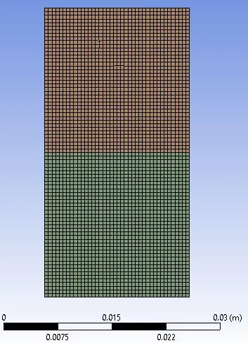
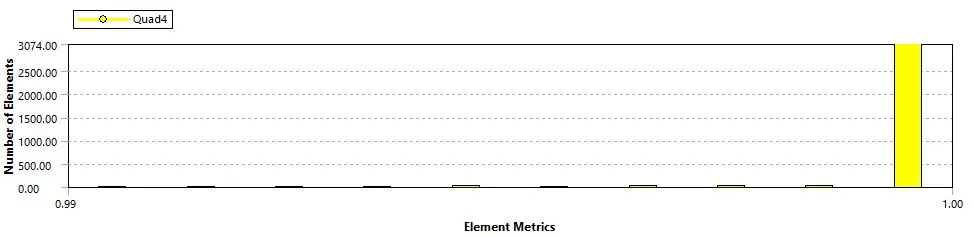
Since the geometry is simple, Hexa mesh elements were used and the resultant mesh had high mesh quality.

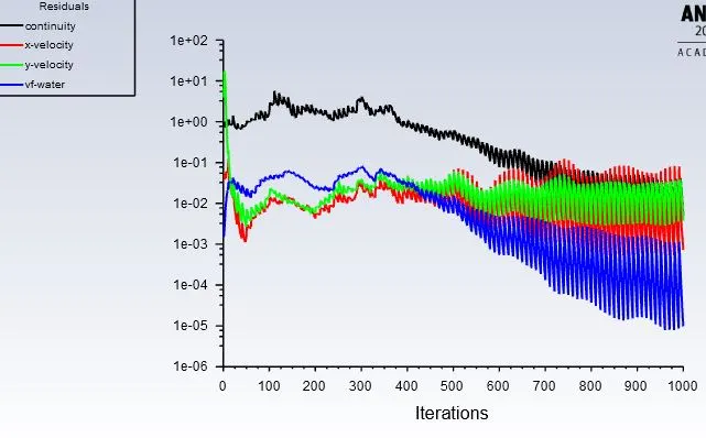
The solution was run for 100 time-steps, with each time-step size of 0.025s, and 10 iterations were performed for each time-step.

2. Mesh element size= 0.4mm

The meshing is done on the given geometry with the mesh element size of 0.4mm. Once the meshing is done, a total of 5151 nodes and 5000 mesh elements were generated.

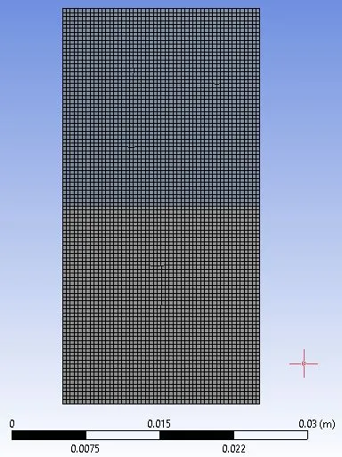
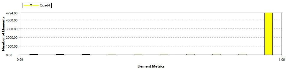
Since the geometry is simple, Hexa mesh elements were used and the resultant mesh had high mesh quality.

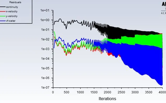
The solution was run for 200 time-steps, with each time-step size of 0.01s, and 20 iterations were performed for each time-step.

3. Mesh element size= 0.25mm

The meshing is done on the given geometry with the mesh element size of 0.25mm. Once the meshing is done, a total of 13041 nodes and 12800 mesh elements were generated.

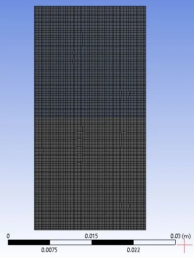
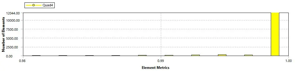
Since the geometry is simple, Hexa mesh elements were used and the resultant mesh had high mesh quality.

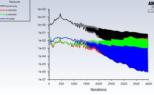
The solution was run for 200 time-steps, with each time-step size of 0.01s, and 20 iterations were performed for each time-step.

Now that the Rayleigh Taylor instability is simulated when the mediums of interaction are air and water, we need to check how this instability changes when the density of the lighter fluid is increased. To simulate this, instead of air as one medium, a user-defined medium is introduced, which has a density of 400Kg/m^3, and viscosity pf 0.001Kg/ms.

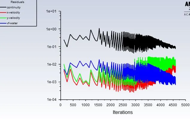
The solution was run for 220 time-steps, with each time-step size of 0.01s, and 20 iterations were performed for each time-step.

As the mesh element size is reduced for the successive simulations, we get a good distribution of the instability. The mixing is more perfect and good and the boundary layers mix better with the decrease in mesh element size. If the mesh element size is decreased and a finer mesh is used, the computational time increases considerably, also the time step size must be reduced with the decrease in the mesh element size, else the solution will diverge. If the time-step size is decreased to a very low value, more time will be taken to perform the simulation, even though the obtained results are more time accurate.

The steady-state approach is not suitable for Rayleigh-Taylor's instability simulation because here we are interested in studying the process of mixing with respect to time, and not much interested in the solution after it has reached the steady-state. As the mixing process is a function of time the transient analysis will give better results and these results are time accurate.

Atwood number:

let,

`rho_(air)=1.225(kg)/m^3`

`rho_(water)= 998.2(kg)/m^3`

`rho_(user)= 400(kg)/m^3`

The Atwood number is given by `A=(rho_1-rho_2)/(rho_1+rho_2)`

`rho_1=` Density of heavier fluid

`rho_2=` Density of lighter fluid

1. Atwood number with air and water as the mediums

`A=(998.2-1.225)/(998.2+1.225)=0.9975`

2. Atwood number with user-defined fluid and water as the mediums

`A=(998.2-400)/(998.2+400)=0.4278`

The Atwood number depends upon the densities and will be in the range of 0-1. The Atwood number for air-water mixing is nearly 1 thus the mixing is quite fast and takes lesser time to come to steady-state. The Atwood number for water and the user-defined material is 0.42, hence the mixing is slower and it takes more time to come to the steady-state than the air-water mixture.

Conclusions:

1. The transient-state analysis is used to perform this simulation since we are interested in time accurate results and not only in the solution once it has reached the steady-state.
2. When a finer mesh is used to perform this analysis, a good distribution of instability is obtained than if a coarse mesh is used. But by doing so, the computation time increases considerably, since the solution needs to be run for a higher number of iterations. With the increase in the number of mesh elements, the time step size must also be reduced, else the solution may diverge.
3. The Atwood number is a dimensionless number in fluid dynamics used in the study of hydrodynamic instabilities in density stratified flows. The Atwood number depends upon the densities and will be in the range of 0-1. Higher the Atwood number, the faster the fluids mix and will attain steady-state.