Modeling and simulation of flow over an Ahmed body
Aim:
To simulate the flow over the Ahmed body having a slope of 35 degrees at the rear and compare the results obtained with the experimental data, and draw suitable conclusions.
Theory:
The Ahmed body is a generic car body (a simplified vehicle model). The airflow around the Ahmed body captures the essential flow features around an automobile and was first defined and characterized in the experimental work of Ahmed. Although it has a very simple shape, the Ahmed body allows us to capture characteristic features that are relevant to bodies in the automobile industry. This model is also used to describe the turbulent flow field around a car-like geometry. Once the numerical model is validated, it is used to design new models of the car.
Geometry:
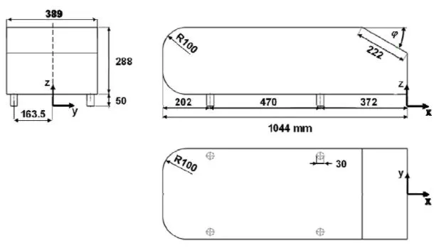
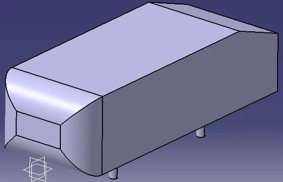
The required Ahmed body geometry was modeled using the CatiaV5 software which is quite popular among CAD softwares. The model specifications are given in the draft, the simple geometrical shape has a length of 1.044 meters, a height of 0.288 meters, and a width of 0.389 meters. It also has four cylindrical legs attached to the bottom of the body of length 50mm and diameter 30mm and the rear surface has a slant that falls off at 35 degrees.
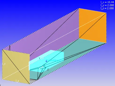
This model is enclosed within a box (virtual wind tunnel) to simulate the flow over Ahmed body. Let the length of the Ahmed body be 'L', then the virtual wind tunnel specifications are as follows; height= 2L from the bottom face of the 4 cylinders of the Ahmed body to the top of the virtual wind tunnel, width= 2L from the center, length= 10L, where the inlet is placed at a distance of 3L from the front face of the Ahmed body, and the outlet is placed at a distance of 6L from the rear face of the Ahmed body.
Once the geometry was created, it is saved in STL format and is exported to Converge CFD.
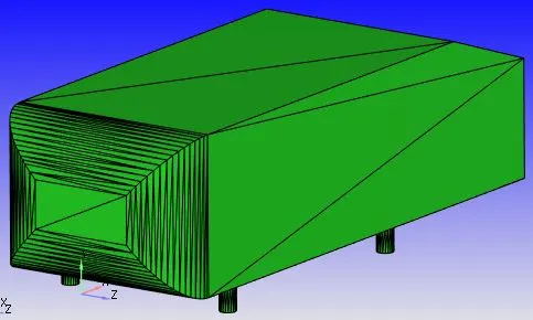
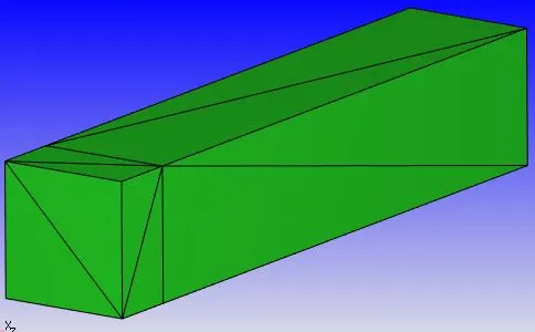
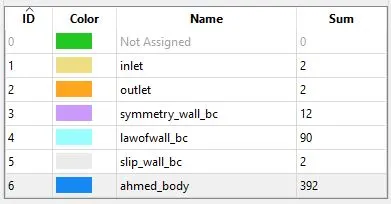
In Converge CFD, the boundaries are named as follows:
Calculations:
Since the Ahmed body is a simplified car model, the bottom surface of the virtual wind tunnel is a wall with either no-slip or law of wall boundary condition. Due to this, there is a formation of a boundary layer as it passes over the Ahmed body. The experimental data available requires a boundary layer thickness of 30mm at a distance of 400mm in front of the front face of the Ahmed body.
Reynolds number, Re=`(rho*v*x)/mu`---(1)
Where,
`rho=`density of air= 1.225 kg/m^3
v= flow velocity= 40m/s
x= Length of the flat plate(bottom wall where the Ahmed body is resting)
`mu=`dynamic viscosity of air= 1.846e-5 kg/(ms)
Boundary layer thickness, `delta=(0.382*x)/(Re)^0.2`---(2)
We know that boundary layer thickness= 30mm
Substituting (1) in (2) and solving for x, we get,
`delta=(0.382*x)/((rho*v*x)/mu)^0.2`
`0.03=(0.382*x^0.8)/(1.225*40)^0.2*(1.846*10^-5)^0.2`
x= 1.678m.
Hence the length of the flat plate (here wall) must be 1.678m to obtain a boundary layer thickness of 30mm. But we want a boundary layer thickness of 30mm, at a distance of 400mm in front of the front face of the Ahmed body, hence the length of the plate must be extended by 400mm to achieve this requirement.
Therefore the length of the plate in front of Ahmed body= 1.678+0.4= 2.078m.
Since we have already provided the distance from the inlet to the front face of the Ahmed body as 3L(3.132m), the excess length of the wall from the inlet(3.132-2.078=1.054m) can be considered as a slip wall. By doing so the boundary layer does not form over the slip wall but begins to form once the flow reaches near the no-slip/law of the wall boundary condition.
Calculation of start time and end time for transient state simulation:
The inlet velocity= 40m/s
The length of the virtual wind tunnel= 10.44m
The time taken by the fluid to move from inlet to outlet= 10.44/40= 0.261s
Suppose we want to simulate the flow for 3-4 times this value, then 0.261x4~ 1s
Case setup:
1. Run parameters:
Solver= transient, time-based simulation
Simulation mode= full hydrodynamic
Gas flow solver= compressible
2. Simulation time parameters:
Start time= 0s
End time= 1s
Initial time-step= 1e-6s
Minimum time-step= 1e-6s
Maximum time-step= 1s
Maximum convection CFL limit= 1
3. Solver parameters:
Navier-Stokes solver scheme= PISO
Navier-Stokes solver type= Density-based
4. Regions and initialization:
Region0:
Velocity(x, y, z)= (40, 0, 0)m/s
Temperature= 300K
Pressure= 101325Pa
Species= air
5. Boundary:
a. Inlet
Inflow boundary condition
Velocity(x, y, z)= (40, 0, 0)m/s
Pressure= Zero normal gradient(Neumann BC)
Temperature= 300K
Species= air
b. Outlet
Outflow boundary condition
Pressure= 101325Pa
Velocity= Zero normal gradient (Neumann BC)
Species backflow= air
Temperature backflow= 300K
c. Symmetry wall
Symmetry boundary condition
d. Law of wall
Stationary wall boundary condition(law of wall)
Law of wall boundary condition is used rather than no-slip boundary condition since the law of wall boundary condition gives more accurate results when a coarse mesh is used, whereas, the no-slip boundary condition gives more accurate results if a finer mesh is used. This is mainly because for the no-slip boundary condition, the solver considers the first cell adjacent to the wall as zero velocity magnitude. When the law of wall boundary condition is used, the solver uses the law of the wall assumption for velocity in the log-log layer tries to estimate the flow properties near the walls. Hence it gives less error when a coarse mesh is used.
e. Slip wall
Stationary wall boundary condition (slip wall)
The slip wall boundary condition does not produce any boundary layer effects. This boundary condition is used since it is the requirement to get a boundary layer thickness of 30mm at a distance of 400mm in front of the front face of the Ahmed body. The plate length is calculated, and the excess length is provided as a slip wall boundary condition.
f. Ahmed body
Stationary wall boundary condition(law of wall)
6. Turbulence modeling
K-omega SST turbulence model
7. Grid control:
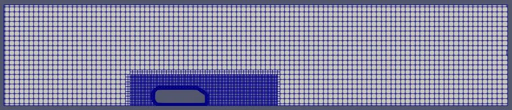
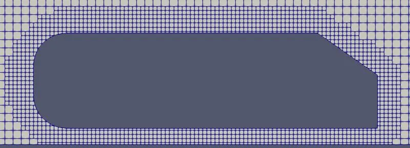
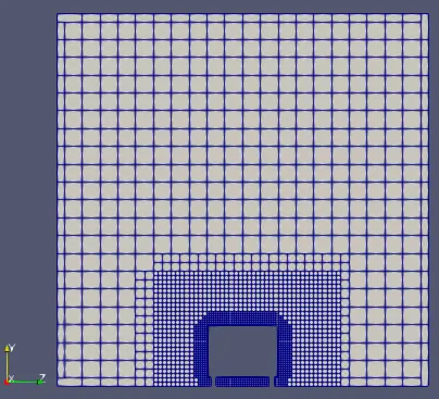
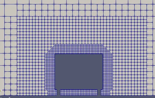
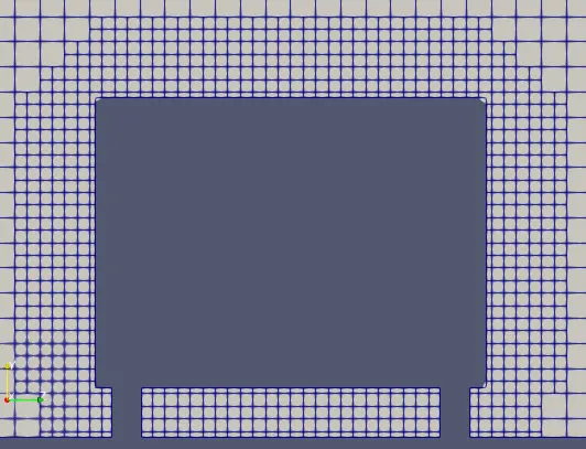
Base grid size(x, y, z)= (0.1 0.1, 0.1)m
Fixed embedding:
a. Embedding1
Entity type= box enclosing the Ahmed body
Dimensions(x, y, z)= (3, 0.6, 1)m
Mode= permanent
Scale= 2
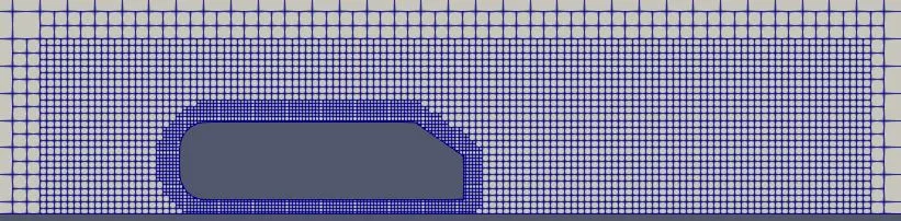
b. Embedding2
Entity type= boundary
Boundary ID= Ahmed body
Mode= permanent
Scale= 3
Embed layers= 5
8. Output files:
Wall output= boundaries only
Time interval for writing 3D output data files= 0.01s
Time interval for writing text output= 1e-6s
Time interval for writing restarting output= 0.01s
Results:
Mesh:
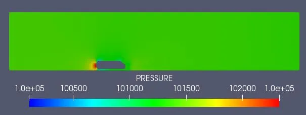
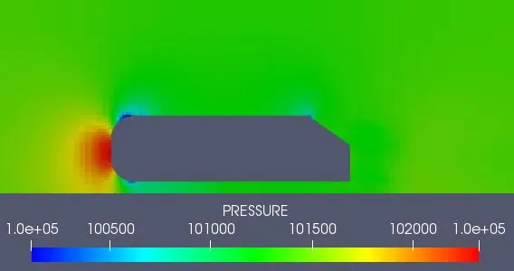
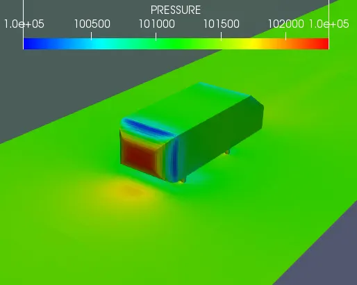
Pressure contours:
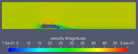
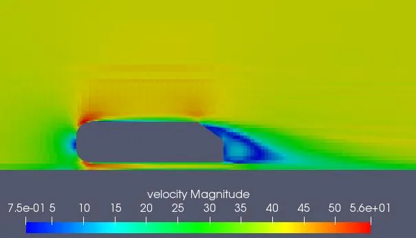
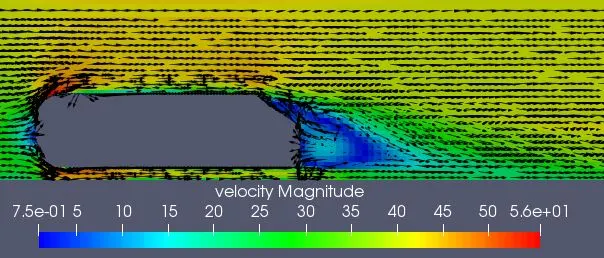
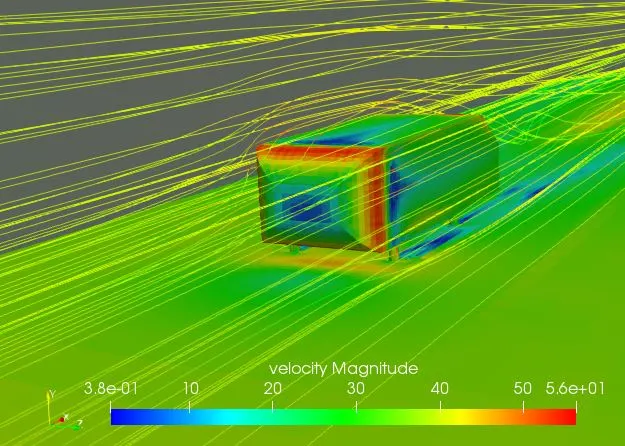
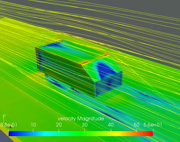
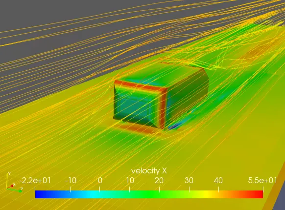
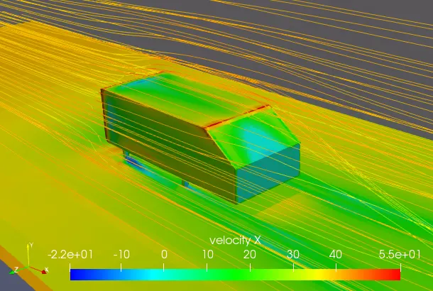
Velocity contours:
Cell count:
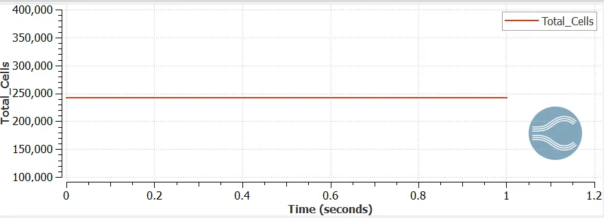
A total of 242237 cells were generated.
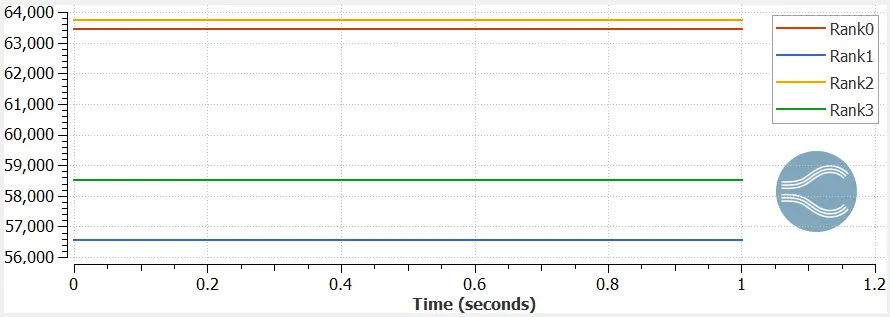
4 processors were used to solve the problem, the cell distribution among the processors are as follows:
Rank0= 63436
Rank1= 56562
Rank2= 63724
Rank3= 58515
Pressure force:
a. Drag:
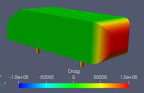
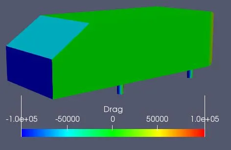
The drag contours were obtained in paraview. First the Ahmed body is extracted from the geometry, then the surface is extracted from this body so that surface normals can be generated from the extracted surface. Drag can be calculated using the calculator. The formula for drag is given by the product of pressure force with normals in the x-direction.
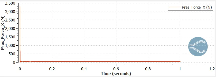
The drag force is estimated by taking the average value of drag force from time 0.8s to 1s. The estimated drag force converges to 39.21497N
Drag, D= `1/2rhov^2SC_d`
Where,
`rho=` density of air= 1.225kg/m^3
v= flow velocity= 40m/s
S= planform area= 0.288x0.389= 0.112032m^2
Cd= coefficient of drag
`C_d=(2*D)/(rho*v^2*S)=(2*39.21497)/(1.225*40^2*0.112032)=0.3571`
b. Lift
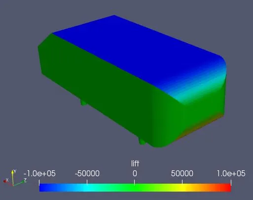
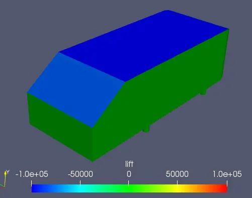
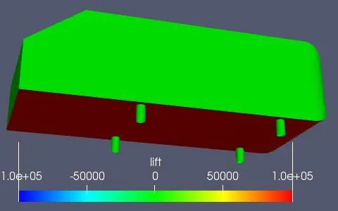
The lift contours were obtained in paraview. First the Ahmed body is extracted from the geometry, then the surface is extracted from this body so that surface normals can be generated from the extracted surface. Lift can be calculated using the calculator. The formula for lift is given by the product of pressure force with normals in the y-direction.
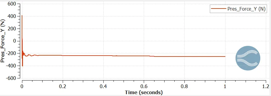
The lift force is estimated by taking the average value of drag force from time 0.8s to 1s. The estimated lift force converges to -251.522N. The negative sign indicates that the Ahmed body produces lift force in the opposite direction, this increases the overall weight force of the body when the air is flowing over it at a velocity of 40m/s. In automobiles, it is highly recommended to have higher values of negative lift since it increases the traction force between the tires and the road, which in turn improves its overall performance.
Lift, L= `1/2rhov^2SC_l`
`C_l=(2L)/(rho*v^2*S)=-(2*251.522)/(1.225*40^2*0.112032)=-2.2909`
Yplus:
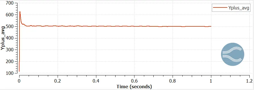
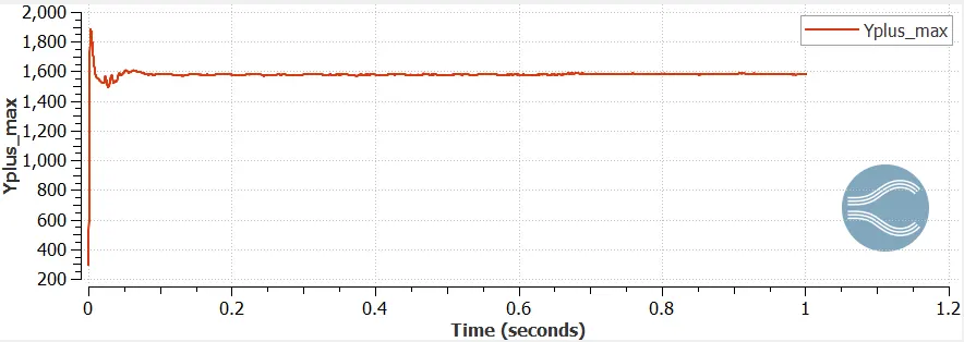
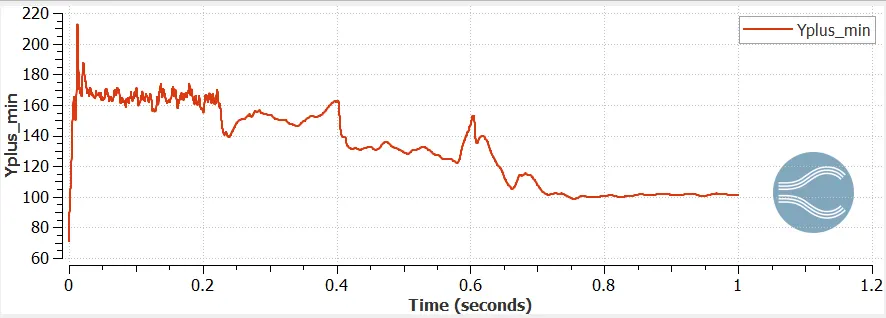
The mean value of yplus term converges at around 500, and it ranges from approximately 100 to 1600 at different locations towards the end of simulation.
Comparison of results obtained with the experimental data:
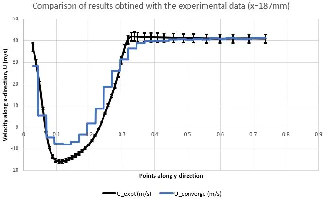
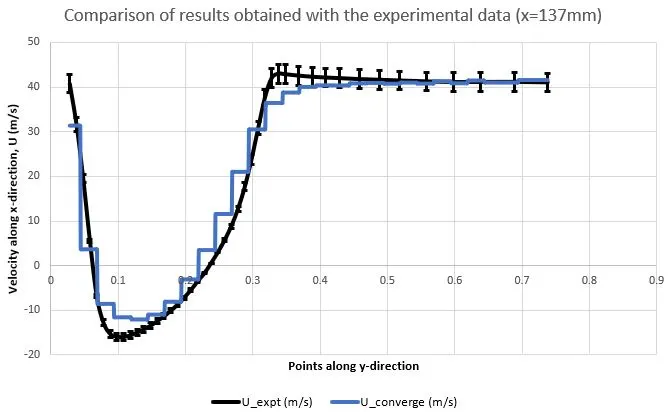
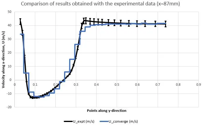
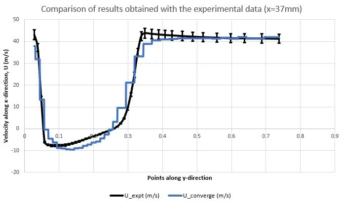
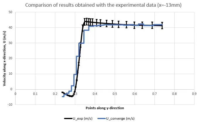
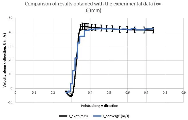
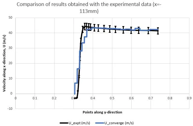
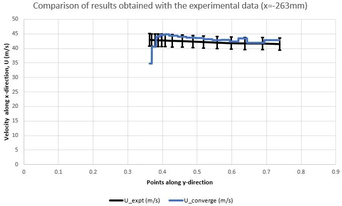
The simulated results are compared with the available experimental data using multiple line probes at different locations along the x-direction. These line probes monitor the velocity along the x-direction(U) at different points along the line. The results obtained from the simulation are plotted against the experimental data, and the following results were obtained.
1. Line probe location= 187mm
2. Line probe location= 137mm
3. Line probe location= 87mm
4. Line probe location= 37mm
5. Line probe location= -13mm
6. Line probe location= -63mm
7. Line probe location= -113mm
8. Line probe location= -263mm
Normalized velocity plots over Ahmed body:
The above plots give the trend of x-velocity magnitude with respect to different y-locations on the given line probe, but it is difficult to compare the results obtained by 2 or more line probes simultaneously. To make it possible to compare the results obtained by multiple line probes simultaneously, the velocity component is normalized, ie, dividing the velocity term at a particular point by the maximum velocity magnitude onthat line probe. By doing so, the velocity component is non-dimensionalized, and the same can be done for remaining line plots and also for experimental data, and finally, the plot obtained results are plotted on a sheet. This process can be achieved by writing a simple octave program, and the resulting plot is as follows:
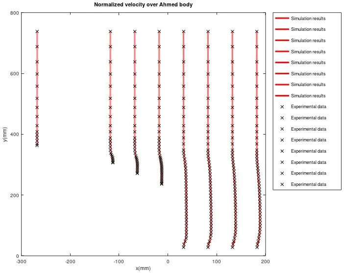
The above results show the variation of x-velocity magnitude at different line probes along the x-direction. Here, the comparison of the results obtained using different line probes can be done simultaneously, also, the simulated results can be compared with the experimental data for different line probes.
Conclusions:
Hence, the flow over the Ahmed body was simulated using Converge CFD and the obtained results were compared with the experimental data and the following conclusions can be drawn:
- As the air moves past the Ahmed body, there is a recirculation zone behind the Ahmed body. This is due to a drop in static pressure.
- This simulation was performed using a base mesh size of 0.1m, with box and boundary embedding of scale 2 and 3 respectively. The total number of mesh elements generated is 242237, which is solved using 4 processors. The average Yplus value converges to around 500. The accuracy of the solution can be improved by further refining the mesh thereby reducing the Yplus value.
- The lift and drag coefficient value calculated using the simulated data was found to be 0.3571 and -2.2909 respectively. The negative value of lift coefficient indicates that the lift is acting in the negative y-direction. It is desirable in automobiles to have negative lift, since this force exerts higher downward force, which in turn increases the traction between the road and tires of the vehicle, due to which the performance of that vehicle improves.
- Line probes are drawn at different locations along the x-direction, and the simulated results were compared with the experimental data. It is found that the simulated results are not within the 5% error limit at some locations. This is due to coarse mesh used to perform the simulation which results in the average yplus value to convrge around 500. To get more accurate results, the element size must be reduced substantially, such that the resulting yplus value lies within the range of 30 to 100. Neverthless, the simulated results follow the same trend line as that of the experimental data.
- The velocity magnitude can be normalized so as to compare the results obtained by 2 or more lineplots simultaneously on a single plot.