SIMPLE PENDULUM ODE USING MATLAB
AIM
Your objective is to write a program that solves the following ODE. This ODE represents the equation of motion of a simple pendulum with damping
Use L=1 metre, m=1 kg, b=0.05, g=9.81 m/s2. Simulate the motion between 0-20 sec, for angular displacement=0,angular velocity=3 rad/sec at time t=0.
PRE-REQUISITES
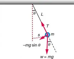
A pendulum is essentially a weight that is hung from a fixed point. It is placed in such a way that it allows the device to swing freely to and fro. The pendulum bob of a simple pendulum is treated as a point mass. Further, the string from which it’s hanging is of negligible mass and is an example of simple harmonic motion.
FUNCTIONS USED
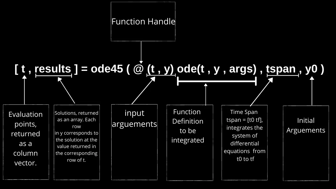
What is ODE45? :- Ode45 is a function in matlab that solves ordinary or partial differential equations using a numerical method. The numerical method in question here is the 4th order Runge Kutta method.
How does ODE45 works? :- The function ode45 takes 3 inputs. The 3 inputs are the function to be integrated, the time span and the initial conditions.
The syntax is:-
CALCULATIONS
Let `theta = theta1 implies (d(theta))/dt = theta2 to eqn1`
On double differentiating eqn1 `(d^2theta)/dt^2 = (d^2theta1)/dt^2 =d/dt((d(theta1))/dt) = (d(theta2))/dt to eqn2`
Pendulum ODE in terms of `theta1 implies (d^2(theta1))/dt^2 + [(b/m)*(d(theta1))/dt]+[(g/L)*sin(theta1) =0]`
Submitting eqn1 & eqn2 in the above eqn `implies (d(theta2))/dt +[(b/m)*theta2]+[(g/L)*sin(theta1)]=0`
Now, `(d(theta2))/dt = [(-b/m)*theta2]-[(g/L)*sin(theta1)] to eqn3`
The eqn1 & eqn3 written in the form of matrix as `d/dt[[theta1],[theta2]] = [[theta2],[[(-b/m)*theta2]-[(g/L)*sin(theta1)]]]`
Now, we will define the LHS of the above eqn. to a single array variable. `theta` for the programs consistency,(i.e) `theta=d/dt[[theta1],[theta2]]`
NOTATIONS
g `to`gravity in m/s2,
L `to`ength of the pendulum in m,
m `to`mass of the ball in kg,
b `to`damping coefficient
PROCEDURE
- The required inputs are defined as shown.
% REQUIRED INPUTS
b=0.05;                           % damping coefficent
g=9.81;                           % gravity (m/sec^2)
l=1;                              % length of the pendulum (m)
m=0.1; % mass of pendulum (kg)- The sigle array variable to store the angular displacement & angular velocity is defined as shown. The former is kept as 0.
%INITIAL CONSITION
theta=[0;5];                                  % angular displacement & angular velocity
% is defineded in this array variable,theta- Now we need the time limits.This can be provided as a vector of 2 values, the initial and final time or with a spacing using the linspace function.
%TIME LIMITS
time=linspace(0,20,500); % The time limits for ode45- Then define an bjective function,(i.e. ode_func()). Here we will define the converted 2nd order pendulum ODE's. They are the eqn1 and eqn3 in the CALCULATION. This objective function intakes as, the current time (t), (theta) would be the value of the function at the previous time step and other arguements such as b,g,L,M. The code is as shown:-
function [dtheta_dt] = ode_func(t,theta,b,g,l,m);                  % the function with input arguements is defined
    theta1 = theta(1);                                             % assisgning the initial angular displacement value,(i.e. 0) from array theta in the main program to the new variable,theta1
    theta2 = theta(2);                                             % assisgning the initial angular velocity value,(i.e. 3) from array theta in the main program to the new variable,theta2
    dtheta1_dt = theta2;                                           % the ODE eqn1 is defined
    dtheta2_dt = -(b/m)*theta2 - (g/l)*sin(theta1);                % the ODE eqn2 is defined
    dtheta_dt = [dtheta1_dt;dtheta2_dt];                           % THE 2 ode are assigned as a coloumn vector to a new array variable (i.e.dtheta_dt)
end- Then, we will call this above function (i.e. ode_func(t,theta,b,g,l,m)), with the help of ode45 numerical solver. The function ode45 is defined with the anonymous function and takes 3 inputs. The 3 inputs are the function to be integrated, the time span and the initial conditions.
% DECLARATION OF NUMERICAL SOLVER-"ODE45"
[t,results] = ode45(@(t,theta) ode_func(t,theta,b,g,l,m),time,theta);- The output till the above state ment will be two coloumn vectors:-
- t→a coloumn vector of size (500*1)
- results→a coloumn vector of size (500*2)
output:-
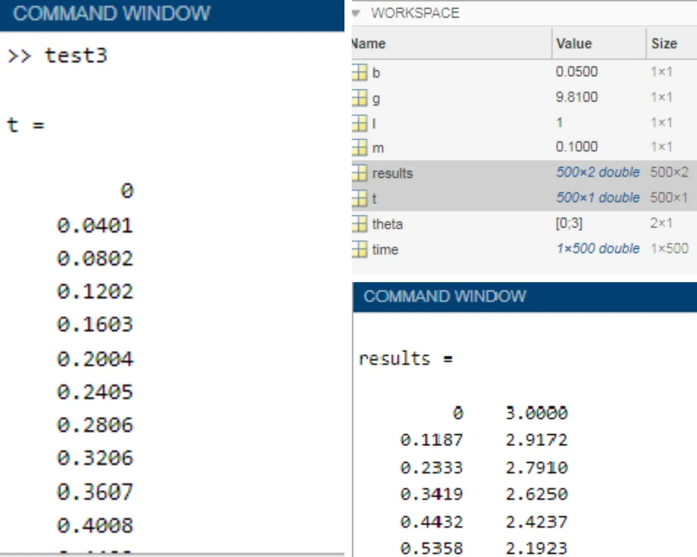
- Note:- The first coloumn of results is angular displacement & the second is angular velocity.
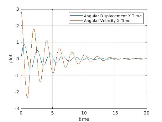
- Now we will plot the variation of angular displacement & angular velocity with time.
% PLOTTING
plot(t,results(:,1));             % the time & angular displacment variation is plotted
hold on                           % to make the the two plots in in figure
plot(t,results(:,2));             % the time & angular velocity variation is plotted
ylabel('plot');                   % x-axis is labelled
xlabel('time');                   % y-axis is labelled
grid on;                          % make plot with grid
output:-
- Now comes the animation rendering part.
- Here for loop is executed, so that automatically, plots for different coordinates of pendulum are stored.
% RENDERING OF PENDULUM


for i=1:length(results(:,1))                                     % for iterating the position of pendulum at each time frame

    x0=0;                                                        % x coordinate of the pivoted end of the pendulum
    y0=0;                                                        % y coordinate of the pivoted end of the pendulum

    x1=l*sin(results(i,1));                                      % x cordinate of the non-pivoted end
    y1=-l*cos(results(i,1));                                     % y cordinate of the non-pivoted end

    plot([-0.5,0.5],[0,0],'linewidth',3,'color','r');            % plots the pivotting line to which the pendulum is oscillating
    hold on                                                      % makes all the plots in one figure without ommitting anything
    plot([x0 x1],[y0 y1],'linewidth',2,'color','g');             % plots the pendulum length
    plot(x1,y1,'o','MarkerSize',20,'markerfacecolor','b');       % plots the bob of the pendulum

    grid on                                                      % open up the grid for the graph
    axis([-1.5 1.5 -1.5 0.5])                                    % makes the axis fixed, if this is not there, then the axis of each plot will vary according to the coordinates
    pause(0.01)                                                  % pauses the iteration for 0.001 seconds
    hold off

    M(i) = getframe(gcf);                                       % stores all the iterations as frames & stored in the array M

end- Then atlast the pendulum motion is made into a video file.
% CREATING THE MOVIE

movie(M)
videofile = VideoWriter('pendulem_animation.avi','uncompressed AVI')       % create an AVI file object ideowriter
open(videofile)                                                            % Open the VideoWriter object
writeVideo(videofile,M)                                                    % write the movie
close(videofile)
PROGRAM
function [dtheta_dt] = ode_func(t,theta,b,g,l,m);                  % the function with input arguements is defined
    theta1 = theta(1);                                             % assisgning the initial angular displacement value,(i.e. 0) from array theta in the main program to the new variable,theta1
    theta2 = theta(2);                                             % assisgning the initial angular velocity value,(i.e. 3) from array theta in the main program to the new variable,theta2
    dtheta1_dt = theta2;                                           % the ODE eqn1 is defined
    dtheta2_dt = -(b/m)*theta2 - (g/l)*sin(theta1);                % the ODE eqn2 is defined
    dtheta_dt = [dtheta1_dt;dtheta2_dt];                           % THE 2 ode are assigned as a coloumn vector to a new array variable (i.e.dtheta_dt)
end
% matlab program to solve ode of pendulum
% REQUIRED INPUTS
b=0.05; % damping coefficent
g=9.81; % gravity (m/sec^2)
l=1; % length of the pendulum (m)
m=1; % mass of pendulum (kg)
%initial conditions % angular displacement & angular velocity
theta=[0;3]; % is defineded in this array variable,theta
%time points
time=linspace(0,20,500); % The time limits for ode45
% DECLARATION OF NUMERICAL SOLVER-"ODE45"
[t,results] = ode45(@(t,theta) ode_func(t,theta,b,g,l,m),time,theta);
% PLOTTING
plot(t,results(:,1)); % the time & angular displacment variation is plotted
hold on % makes all the plots in one figure without ommitting anything
plot(t,results(:,2)); % the time & angular velocity variation is plotted
ylabel('plot'); % x-axis is labelled
xlabel('time'); % y-axis is labelled
legend("Angular Displacement X Time","Angular Velocity X Time") % the curves are labelled
grid on; % make plot with grid
% RENDERING OF PENDULUM
for i=1:length(results(:,1)) % for iterating the position of pendulum at each time frame
x0=0; % x coordinate of the pivoted end of the pendulum
y0=0; % y coordinate of the pivoted end of the pendulum
x1=l*sin(results(i,1)); % x cordinate of the non-pivoted end
y1=-l*cos(results(i,1)); % y cordinate of the non-pivoted end
plot([-0.5,0.5],[0,0],'linewidth',3,'color','r'); % plots the pivotting line to which the pendulum is oscillating
hold on % makes all the plots in one figure without ommitting anything
plot([x0 x1],[y0 y1],'linewidth',2,'color','g'); % plots the pendulum length
plot(x1,y1,'o','MarkerSize',20,'markerfacecolor','b'); % plots the bob of the pendulum
grid on % open up the grid for the graph
axis([-1.5 1.5 -1.5 0.5]) % makes the axis fixed, if this is not there, then the axis of each plot will vary according to the coordinates
pause(0.01) % pauses the iteration for 0.001 seconds
hold off
M(i) = getframe(gcf); % stores all the iterations as frames & stored in the array M
end
% CREATING THE MOVIE
movie(M)
videofile = VideoWriter('pendulem_animation.avi','uncompressed AVI') % create an AVI file object ideowriter
open(videofile) % Open the VideoWriter object
writeVideo(videofile,M) % write the movie
close(videofile) % close the fileANIMATION VIDEO
RESULT
- The plot between angular displacement & time is successfully carried out.
- The plot between angular velocity & time is successfully carried out.
- The animation of pendulum oscillation is successfully careried out.
INFERENCES
- Understanding Anonymous Functions in MATLAB `to` https://skill-lync.freshdesk.com/support/solutions/articles/43000580974
- Understanding ODE45 `to` https://skill-lync.freshdesk.com/support/solutions/articles/43000580976-understanding-ode45