CURVE FITTING USING MATLAB INBUILT FUNCTION & MATLAB OPTIMIZATION TOOL
AIM
Understanding CURVE FITTING using MATLAB inbuilt function and MATLAB Optimization Tool
OBJECTIVE 1 →→ Write code to fit a linear and cubic polynomial for the Cp (Specific Enthalpy) data. Plot the linear and cubic fit curves along with the raw data points. Title and axes labels are a must, legends could be shown if necessary.
OBJECTIVE 2 →→ Explain the parameters used to measure the fitness characteristics for both the curves.
OBJECTIVE 3 →→ Write a code to show splitwise method.
PRE-REQUISITES
There are methods of analysing a set of data and creating a function out of it, that describes the best of its values.
They are :-
1. INTERPOLATION →→ When we predict values that fall within the range of our data.
2. EXTRAPOLATION →→ When we predict the values of a variable beyond the range of our data.
3. CURVE FITTING →→
In our schools, we used various means, such as histograms, frequency polygons and ogives, to visualise our data. These are very useful tools to depict univariate data, i.e. data with only one variable such as the height of learners in a class.
Last year we also learnt about a visual tool called scatter plots. Scatter plots are a common way to visualise bivariate data, i.e. data with two variables. This allows us to identify the direction and strength of a relationship between two variables.
We identify the nature of a relationship between two variables by examining if the points on the scatter plot conform to a linear, exponential, quadratic or some other function. The process of fitting functions to data is known as curve fitting.
We simply want a function that is a good fit (typically a best fit in some sense) to the original data points. With curve fitting the approximating function does not have to pass through the original data set.
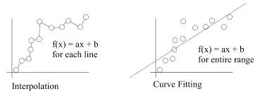
Why do we curve fit ? ⇒ For many applications you need to find a mathematical formula that adheres to a set of data points. The curve helps you understand how your data changes mathematically. it can help in doing additional calculations which may be very complex using original data.
Curve Fitting Functions→→ 1. Optimal Straight Line Polynomial Degree (1)
2. Optimal Polynomial Degree (2,3,...)
IMPORTANT INBUILT FUNCTIONS USED
polyfit(x,y,n) → generates the coefficients of the polynomial, which can be used to model a curve to fit the data.
polyval(p,x) → returns the value of the polynomial p evaluated at x.
PROCEDURE
OBJECTIVE-1 `to` Stepwise solution to code any curve fit:-
- The first step is to load the file in the MATLAB. Only if the MATLAB accesses the file, it can make those calculations. Here the file name is "data".
% PREPARING THE FILES
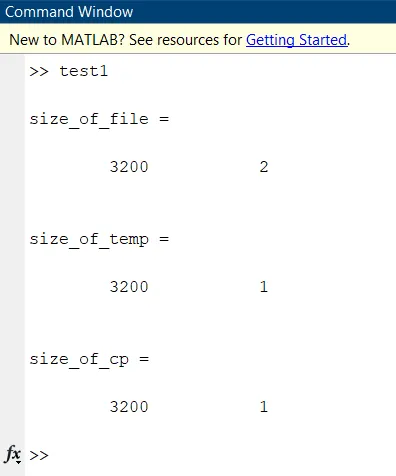
% file "data" has 3200 X 2
cp_data = load('data');                             % The file named "data" is loaded and stored in the variable, cp_data
size_of_file = size(cp_data)                        % the size of the cp_is calculated
temp = cp_data(:,1);                                % the first coloumn is assigned to variable "temp"
cp = cp_data(:,2);                                  % the first coloumn is assigned to variable "cp"
size_of_temp =  size(temp)                          % size of "temp" is calculated
size_of_cp = size(cp)                               % size of "cp" is calculated
Outout:-
- Now, the curve fit for linear polynomial is carred out. Here the temperature coordinates are same as in the original data file, but the cp values are considered as function values (i.e. cp = p1*temp+p2). Hence they will change, because they depends on the coefficents p1 and p2. Therefore, we will predict the new cp value. It is done using the inbuilt matlab functions- polyfit(), polyval().
% LINEAR FIT
% cp = p1*temp + p2
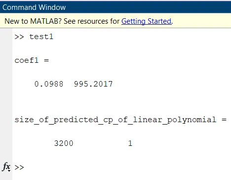
coef1 = polyfit(temp,cp,1)                                       % coefficent of the linear polynomial is calculated
pred_cp1 = polyval(coef1,temp);                                  % the polynomial value "y" is calculated
size_of_predicted_cp_of_linear_polynomial = size(pred_cp1)       % size of variable pred_cp1
Outout:-
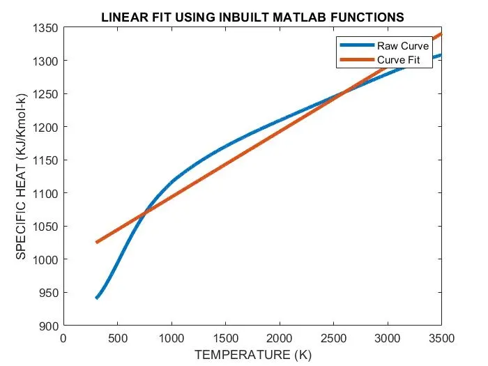
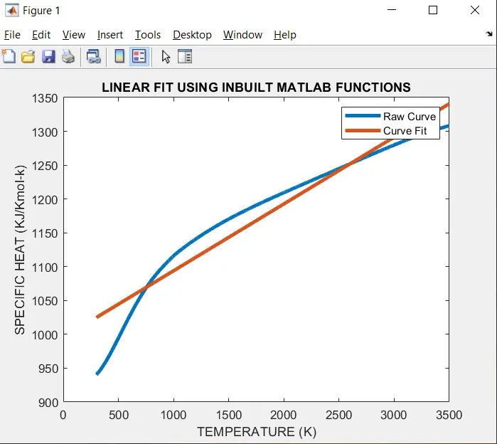
- Then we will plot the curve fit for linear polynomial. Also for better understanding we will compare this linear ploynomial curve fit with the original curve.
% PLOTTING 1- FOR LINEAR POLYNOOMIAL
figure(1)                                           % this will deliver the plots after this command in a new window
plot(temp,cp,'linewidth',3)                         % this gives the original curve using the raw values from the file linear polynomial
hold on                                             % enables overwritting of the plot
plot(temp,pred_cp1,'linewidth',3)                   % this gives the linear curve fit using the inbuilt polyfit() and polyfit()
xlabel('TEMPERATURE (K)')                           % labels the x-axis
ylabel('SPECIFIC HEAT (KJ/Kg)')                     % labels the y-axis
title('LINEAR FIT USING INBUILT MATLAB FUNCTIONS')  % gives the title to the plot
legend("Raw Curve","Curve Fit")                     % labels the curves plotted
Output:-
OBJECTIVE 2 `to` Fitness Characteristics for a Curve Fitting:-
- By seeing the above curves, can you tell the curve fitting carried out is satisfying ? Well, there are some goodness of fit criteria, to assess how well the equation is representing the data points. They are:-
- SSE or (Sum of Squares Due to Error)
- R - Square
- Adjusted R - Square
- (RMSE) or Root Mean Squared Error
- SSE or (Sum of Squares Due to Error) `to`In the above linear curve fit (i.e. not the raw curve),we have some individual errors (i.e. difference in y-coordinate values). SSE is nothing but squaring those arrors & adding them.
i.e. SSE = `sum_(i=1)^n[Err(i)^2]=sum_(i=1)^n[y(i)-(f(x(i)))]^2`
- R - Square `to` It is a scale of defining how good the fit is in explaining the variation of data.
For `R^2`=0→ worst curve fit
`R^2`=1→ best curve fit
`R^2=(SSR)/(SST)`, where SST = SSR + SSE
`SSR=sum_(i=1)^n[f(x(i))-mean]^2`
- Adjusted R - Square `to`It is like normalising R- Square value. It eliminates variations due to insignificant varisbles and considers only the variables that contribute to the real output.
`R^2adj=(((1-R^2)(n-1))/(n-k-1))`, where n`to`Number of datapoints
k`to`the Number of independent variables
- (RMSE) or Root Mean Squared Error `to`It is an estimate of standard deviation of the random component in the data and defined as:-
`RMSE=sqrt(((sum_(i=1)^n)(Err(i))^2)/n)=sqrt((SSE)/n)`where n`to`Number of datapoints
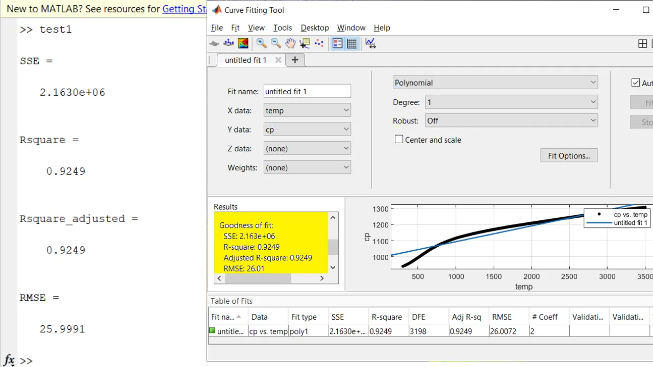
- Now we will check the goodness of fit of linear curve fit.
- For that we define a for loop and define the above formulas.
% GOODNESS FIT CRITERIA FOR LINEAR CURVE FIT
SSE1 = 0;                                           % the initial value of "sum of squares due to error" is kept as 0 for applying in the for loop
SSR = 0;                                            % the initial value of "sum of squares of regression" is kept as 0 for applying in the for loop
SST = 0;                                            % the initial value of SST is kept as 0 for applying in the for loop
sum = 0;                                            % the initial sum value for finding mean from the predicted_cp array
for i=1:length(cp)                                  %
    sum = sum+cp(i);                                % for loop for finding mean value
end                                                 %
mu = sum/length(cp)                                 % the mean value ids obtained
for i=1:length(temp)                                % the for loop for repeated iteration to find SSE,SSR & SST

    SSE1 = SSE1+(cp(i)-pred_cp1(i))^2;              % this will store the SSE1 for the particular index and simultaneously, calculates its own summation
    SSR = SSR+(pred_cp1(i)-mu)^2;                 % this will store the SSR for the particular index and simultaneously, calculates its own summation
    SST = SSR+SSE1;                                 % this will find the respective summation of SSR & SSE1 and simultaneously, calculates its own summaion

end

SSE = SSE1                                          % the summation of SSE1 is stored in SSE
Rsquare=SSR/SST                                     % Rsquare is calculated
n = length(temp);                                   % no: of datapoints
k=1;                                                % no: of independent variables
Rsquare_adjusted =1- [(1-Rsquare)*(n-1)/(n-k-1)]    % Rsquare_adjusted is calculated
RMSE = (SSE/n)^0.5                                  % root_mean_square_error is calculated
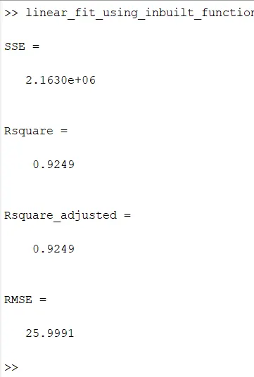
COMMAND WINDOW output for the above code is as shown below. And from the point of validation, the cftool output is also attached.
- Similarly, we will develop MATLAB cding for the cubic curve fit. There will be cubic polynomial inbuilt MATLAB functions to get the coefficents, then we will plot them and compare with the original curve, and then find he goodness fit criteria for cubic polynomial.
% PREPARING THE FILES
% file "data" has 3200 X 2
cp_data = load('data');                             % The file named "data" is loaded and stored in the variable, cp_data
size_of_file = size(cp_data);                                      % the size of the cp_is calculated
temp = cp_data(:,1);                                % the first coloumn is assigned to variable "temp"
cp = cp_data(:,2);                                  % the first coloumn is assigned to variable "cp"
size_of_temp =  size(temp);                                         % size of "temp" is calculated
size_of_cp = size(cp);                                           % size of "cp" is calculated


% CUBIC FIT
% y = (a*(x^3))+(b*(x^2))+(c*(x))+d
coef2 = polyfit(temp,cp,3);                                     % coefficent of the linear polynomial is calculated
pred_cp2 = polyval(coef2,temp);                                 % the polynomial value "y" is calculated


% PLOTTING 2- FOR CUBIC PLYNOMIAL
figure(2)                                           % this will deliver the plots after this command in a new window
plot(temp,cp,'linewidth',3,'color','r')                         % this gives the original curve using the raw values from the file for cubic polynomial
hold on                                             % enables overwritting of the plot
plot(temp,pred_cp2,'linewidth',3,'color','b')                   % this gives the linear curve fit using the inbuilt polyfit() and polyfit()
xlabel('TEMPERATURE (K)')                           % labels the x-axis
ylabel('SPECIFIC HEAT (KJ/Kmol-k)')                     % label the y-axis
title('CUBIC FIT USING INBUILT MATLAB FUNCTIONS')   % gives title to the plot
legend("Raw Curve","Curve Fit")                     % labels the curve plotted


% GOODNESS FIT CRITERIA FOR CUBIC CURVE FIT
SSE1 = 0;                                           % the initial value of "sum of squares due to error" is kept as 0 for applying in the for loop
SSR = 0;                                            % the initial value of "sum of squares of regression" is kept as 0 for applying in the for loop
SST = 0;                                            % the initial value of SST is kept as 0 for applying in the for loop
sum = 0;                                            % the initial sum value for finding mean from the predicted_cp array
for i=1:length(cp)                                  %
    sum = sum+cp(i);                                % for loop for finding mean value
end                                                 %
mu = sum/length(cp)                                 % the mean value ids obtained
for i=1:length(temp)                                % the for loop for repeated iteration to find SSE,SSR & SST

    SSE1 = SSE1+(cp(i)-pred_cp2(i))^2;              % this will store the SSE1 for the particular index and simultaneously, calculates its own summation
    SSR = SSR+(pred_cp2(i)-mu)^2;                   % this will store the SSR for the particular index and simultaneously, calculates its own summation
    SST = SSR+SSE1;                                 % this will find the respective summation of SSR & SSE1 and simultaneously, calculates its own summaion

end

SSE = SSE1                                          % the summation of SSE1 is stored in SSE
Rsquare=SSR/SST                                     % Rsquare is calculated
n = length(temp);                                   % no: of datapoints
k=1;                                                % no: of independent variables
Rsquare_adjusted =1- [(1-Rsquare)*(n-1)/(n-k-1)]    % Rsquare_adjusted is calculated
RMSE = (SSE/n)^0.5                                  % root_mean_square_error is calculated
Output:-
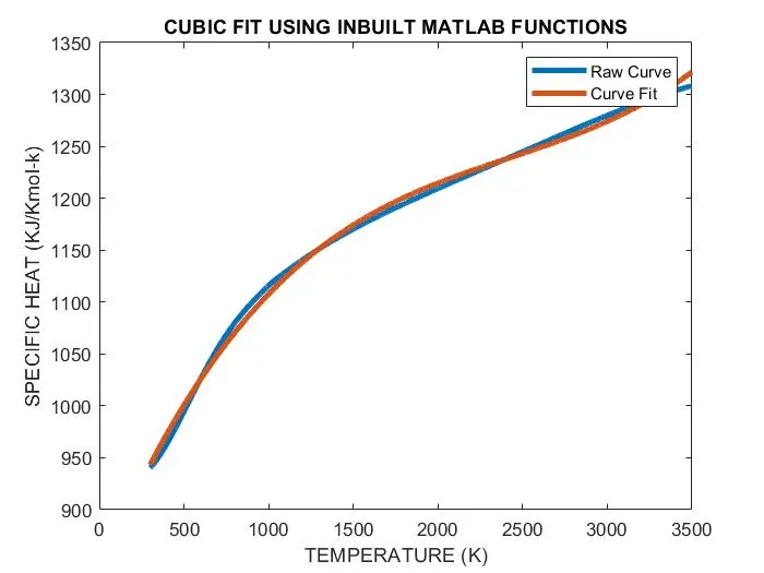
- PLOT
- COMMAND WINDOW and CFTOOL (FOR VALIDATION)
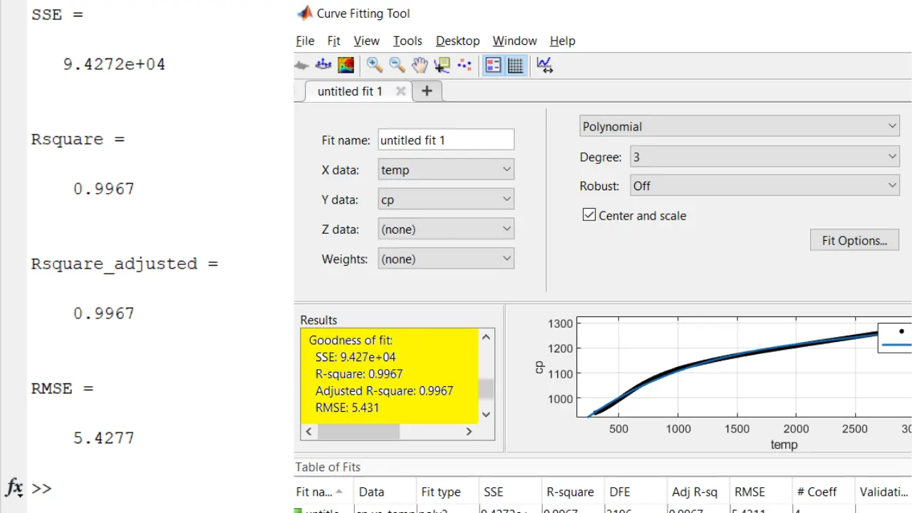
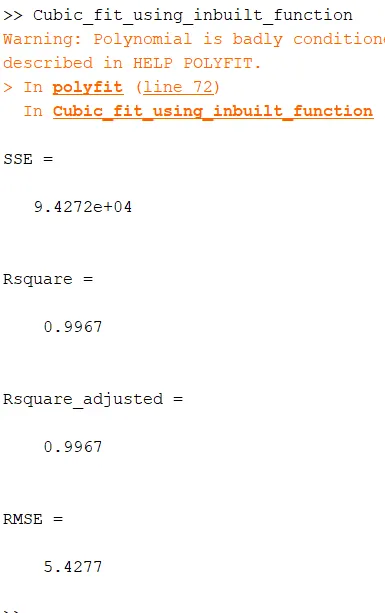
- NOTE:- In the above cftool output, the result needed centering & scaling. Also, in the COMMAND WINDOW, a warning sign was shown as:-
"Warning: Polynomial is badly conditioned. Add points with distinct X values, reduce the degree of the polynomial, or try centering and scaling as described in HELP POLYFIT. "
This signifies that the error formation cannot be negelected. So in those cases we have to use other techniques to reduce the error formation between the datapoints. One such method is SPLITWISE METHOD.
OBJECTIVE 3 `to` Splitwise Curve Fitting Method:-
- SPLITWISE METHOD `to` Here we will divide the data points into a set of intervals and these intervals will be assigned separate polynomials. i have divided the datapoints into 8 intervals as shown in the code.
Output:-
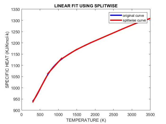
- In the above splitwise curve fitting, i have used the linear polynomial.if i use the higher polynomial, then there will be warning sign in the COMMAND WINDOW. So it means that based on the datapoints, the linear curve fit using the splitwise method is the best fit for the given datapoints.
NOTE:- this above output is not exactly covering the original curve, rather it is lagging in superimposing it. Hence it is not a perfect fit, but the best fit for the datapoints.
PROGRAM
OBJECTIVE 1
1. Linear Polynomial Curve Fit
% PREPARING THE FILES
% file "data" has 3200 X 2
cp_data = load('data');                             % The file named "data" is loaded and stored in the variable, cp_data
size_of_file = size(cp_data);                                      % the size of the cp_is calculated
temp = cp_data(:,1);                                % the first coloumn is assigned to variable "temp"
cp = cp_data(:,2);                                  % the first coloumn is assigned to variable "cp"
size_of_temp =  size(temp);                                         % size of "temp" is calculated
size_of_cp = size(cp);                                           % size of "cp" is calculated


% LINEAR FIT
% cp = p1*temp + p2
coef1 = polyfit(temp,cp,1);                                      % coefficent of the linear polynomial is calculated
pred_cp1 = polyval(coef1,temp);                                  % the polynomial value "y" is calculated
size_of_predicted_cp_of_linear_polynomial = size(pred_cp1);      % size of variable pred_cp1


% PLOTTING 1- FOR LINEAR POLYNOOMIAL
figure(1)                                           % this will deliver the plots after this command in a new window
plot(temp,cp,'linewidth',3)                         % this gives the original curve using the raw values from the file linear polynomial
hold on                                             % enables overwritting of the plot
plot(temp,pred_cp1,'linewidth',3)                   % this gives the linear curve fit using the inbuilt polyfit() and polyfit()
xlabel('TEMPERATURE (K)')                           % labels the x-axis
ylabel('SPECIFIC HEAT (KJ/Kmol-k)')                     % labels the y-axis
title('LINEAR FIT USING INBUILT MATLAB FUNCTIONS')  % gives the title to the plot
legend("Raw Curve","Curve Fit")                     % labels the curves plotted


% GOODNESS FIT CRITERIA FOR LINEAR CURVE FIT
SSE1 = 0;                                           % the initial value of "sum of squares due to error" is kept as 0 for applying in the for loop
SSR = 0;                                            % the initial value of "sum of squares of regression" is kept as 0 for applying in the for loop
SST = 0;                                            % the initial value of SST is kept as 0 for applying in the for loop
sum = 0;                                            % the initial sum value for finding mean from the predicted_cp array
for i=1:length(cp)                                  %
    sum = sum+cp(i);                                % for loop for finding mean value
end                                                 %
mu = sum/length(cp)                                 % the mean value ids obtained
for i=1:length(temp)                                % the for loop for repeated iteration to find SSE,SSR & SST

    SSE1 = SSE1+(cp(i)-pred_cp1(i))^2;              % this will store the SSE1 for the particular index and simultaneously, calculates its own summation
    SSR = SSR+(pred_cp1(i)-mu)^2;                 % this will store the SSR for the particular index and simultaneously, calculates its own summation
    SST = SSR+SSE1;                                 % this will find the respective summation of SSR & SSE1 and simultaneously, calculates its own summaion

end

SSE = SSE1                                          % the summation of SSE1 is stored in SSE
Rsquare=SSR/SST                                     % Rsquare is calculated
n = length(temp);                                   % no: of datapoints
k=1;                                                % no: of independent variables
Rsquare_adjusted =1- [(1-Rsquare)*(n-1)/(n-k-1)]    % Rsquare_adjusted is calculated
RMSE = (SSE/n)^0.5                                  % root_mean_square_error is calculated
Output:- COMMAND WINDOW & PLOT
2. CUBIC POLYNOMIAL FIT
% PREPARING THE FILES
% file "data" has 3200 X 2
cp_data = load('data');                             % The file named "data" is loaded and stored in the variable, cp_data
size_of_file = size(cp_data);                                      % the size of the cp_is calculated
temp = cp_data(:,1);                                % the first coloumn is assigned to variable "temp"
cp = cp_data(:,2);                                  % the first coloumn is assigned to variable "cp"
size_of_temp =  size(temp);                                         % size of "temp" is calculated
size_of_cp = size(cp);                                           % size of "cp" is calculated


% CUBIC FIT
% y = (a*(x^3))+(b*(x^2))+(c*(x))+d
coef2 = polyfit(temp,cp,3);                                     % coefficent of the linear polynomial is calculated
pred_cp2 = polyval(coef2,temp);                                 % the polynomial value "y" is calculated


% PLOTTING 2- FOR CUBIC PLYNOMIAL
figure(2)                                           % this will deliver the plots after this command in a new window
plot(temp,cp,'linewidth',3,'color','r')                         % this gives the original curve using the raw values from the file for cubic polynomial
hold on                                             % enables overwritting of the plot
plot(temp,pred_cp2,'linewidth',3,'color','b')                   % this gives the linear curve fit using the inbuilt polyfit() and polyfit()
xlabel('TEMPERATURE (K)')                           % labels the x-axis
ylabel('SPECIFIC HEAT (KJ/Kmol-k)')                     % label the y-axis
title('CUBIC FIT USING INBUILT MATLAB FUNCTIONS')   % gives title to the plot
legend("Raw Curve","Curve Fit")                     % labels the curve plotted


% GOODNESS FIT CRITERIA FOR CUBIC CURVE FIT
SSE1 = 0;                                           % the initial value of "sum of squares due to error" is kept as 0 for applying in the for loop
SSR = 0;                                            % the initial value of "sum of squares of regression" is kept as 0 for applying in the for loop
SST = 0;                                            % the initial value of SST is kept as 0 for applying in the for loop
sum = 0;                                            % the initial sum value for finding mean from the predicted_cp array
for i=1:length(cp)                                  %
    sum = sum+cp(i);                                % for loop for finding mean value
end                                                 %
mu = sum/length(cp)                                 % the mean value ids obtained
for i=1:length(temp)                                % the for loop for repeated iteration to find SSE,SSR & SST

    SSE1 = SSE1+(cp(i)-pred_cp2(i))^2;              % this will store the SSE1 for the particular index and simultaneously, calculates its own summation
    SSR = SSR+(pred_cp2(i)-mu)^2;                   % this will store the SSR for the particular index and simultaneously, calculates its own summation
    SST = SSR+SSE1;                                 % this will find the respective summation of SSR & SSE1 and simultaneously, calculates its own summaion

end

SSE = SSE1                                          % the summation of SSE1 is stored in SSE
Rsquare=SSR/SST                                     % Rsquare is calculated
n = length(temp);                                   % no: of datapoints
k=1;                                                % no: of independent variables
Rsquare_adjusted =1- [(1-Rsquare)*(n-1)/(n-k-1)]    % Rsquare_adjusted is calculated
RMSE = (SSE/n)^0.5                                  % root_mean_square_error is calculated
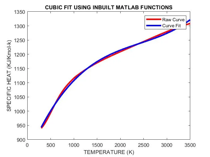
Output:-
Based on the research and programming that i have carried out, let me make something clear:-
- HOW TO MAKE A CURVE FIT PERFECTLY ?
Here when the COMMAND WINDOW gave a warning sign regarding how badly the used polynomial is badly condition, i had to go for alternate solutions to make the curve fit perfectly. i used splitwise technique, wherein the datapoints are divided into certain intervals and applying polynomials to each intervals separately (i.e. finding the coefficents separately and predicting the new function value). Then also i was not able to get the perfect fit, instead i got the best fit for the given datapoints. Other than this i can incease the order of the polynomial or try centering and scaling, either manually or make use of CFTOOL.
- HOW TO GET THE BEST FIT ?
The best fit is one which minimises the error formation between the datapoints and and corresponding function value. Here in the case of splitwise method, i got the output as the best fit, because you can see the red curve does not completely superimpose the blue curve, which implies the fit obtained shows some variation when compared to the original curve.
- WHAT COULD BE DONE TO IMPROVE THE CUBIC FIT ?
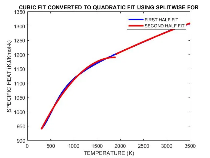
As you know the output shown when datapoints are executed to get the cubic fit. It said that the cubic polynomial is badly condtioned and requires distinct X values or requires centering and scaling using the CFTOOL. So here i will separate the datapoints into two half, wherein, the first half will be from 1 to 1600 and the second half will be from 1600 to 3200. Then the the two halfs are subjected to 2nd degree polynomials using the fit(). Alast we will check the goodness of fit for both the halfs.
Program:-
% MATLAB PROGRAM FOR IMPROVING CUBIC CURVE FITTING

% PREPARING THE FILES
cp_data = load('data');
size(cp_data);

temp = cp_data(:,1);
cp = cp_data(:,2);

temp1 = temp([1:1600]);                                    % the temperature is split from 1 to 1600
temp2 = temp([1600:3200]);                                 % the temperature is split from 1600 to 3200
cp1 = cp([1:1600]);                                        % the cp is split from 1 to 1600
cp2 = cp([1600:3200]);                                     % the temperature is split from 1600 to 3200


coef1 = polyfit(temp1,cp1,2);                              % coefficents of first half of datapoints is calculated
pred_cp1 = polyval(coef1,temp1);                           % the function values(i.e. predicted cp values)of first half of datapoints is calculated

coef2 = polyfit(temp2,cp2,2);                              % coefficents of second half of datapoints is calculated
pred_cp2 = polyval(coef2,temp2);                           % the function values(i.e. predicted cp values)of second halfof datapoints is calculated


% PLOTTING 1- FOR LINEAR POLYNOOMIAL
figure(1)                                                       % this will deliver the plots after this command in a new window
plot(temp,cp,'linewidth',3,'color','b')                         % this gives the original curve using the raw values from the file linear polynomial
hold on                                                         % enables overwriting in the plot
plot(temp1,pred_cp1,'linewidth',3,'color','r')                  % plot for first half of datapoints
plot(temp2,pred_cp2,'linewidth',3,'color','r')                  % plot for second half if datapoints

xlabel('TEMPERATURE (K)')                                                                     % labels the x-axis
ylabel('SPECIFIC HEAT (KJ/Kmol-k)')                                                           % labels the y-axis
title('CUBIC FIT CONVERTED TO QUADRATIC FIT USING SPLITWISE FOR')                             % gives the title to the plot
legend("FIRST HALF FIT","SECOND HALF FIT")
Output:- On executing the above program, no warning output is obtained. Hence we obtained the plot shown below. This way we got the good fit by seperating the datapoints and using the second order polynomial equation
RESULT
1. The curve fit program for linear & cubic polynomial was successfully carried out.
2. Also the respective plots with labels have been carried out
3. The technique to improve cubic polynomial curve fit is successfuly carried out using 2nd order splitwise method.
4. 3 questions based on the research and programming has been answered.
REFERENCES
1. https://www.siyavula.com/read/maths/grade-12/statistics/09-statistics-02
2. https://skill-lync.com/projects/Curve-Fitting-and-criterion-to-choose-best-fit-41860
3. https://skill-lync.freshdesk.com/support/solutions/articles/43000584172