OTTO CYCLE USING MATLAB
AIM
Write a code in Matlab that can solve an otto cycle and make plots for it. Create a PV diagram and find the thermal efficiency of the engine.
PRE-REQUISITES
An Otto cycle is an idealized thermodynamic cycle that describes the functioning of a typical spark ignition piston engine. It is the thermodynamic cycle most commonly found in PETROL engines.
Thes engines:-
- Intake stroke, gasoline vapor and air drawn into engine (suction stroke) (
 ).
). - The fguel gets compressed at high temperature and pessure (Compression stroke) (
 ).
). - Spark is initiated (Combustion stroke) (
 ).
). - The gases get expanded (Power stroke) (
 ).
). - Exhaust gase passes through the outlet valve (Exhaust stroke) (
 )
)
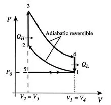
GOVERNING EQUATIONS
- Isentropic Compression & Expansion`implies`(1`to`2)&(3`to`4)`implies P*V^gamma=constant`
- Isochoric heat addition & Rejection`implies`(2`to`3)&(4`to`1)`implies(P/T)=constant`
- Ideal Gas Equation`implies(P*V)/T=constant`
- Compression Ratio`implies(Vs + Vc)/(Vc)`
Change of volume inside the engine combustion chamber:-
`(V/(Vc))=1+(1/2)(CR-1)(R+1-Cos(theta)-sqrt(R^2-Sin(theta)^2))`
Thermal Efficiency `implies 1-(1/(CR)^(gamma-1))`
NOTATIONS
P `to` Pressure (Pa), V `to` Volume (m^3), T `to`Temperature (K)
CR `to` Compression Ratio, y`to`Specific Heat Ratio
Vc `to` Clearance Volume (m^3), Vs`to`Swept Volume (m^3)
R `to` Ratio of length of connecting rod to the crank pin radius, a `to` Crank Pin Radius (m)
PROCEDURE
- The first and the foremost step is to define the input values. Here it is the engine parameters.
% ENGINE PARAMETRES
bore=0.1;                              % bore diameter (m)
stroke=0.1;                            % stroke length (m)
connecting_rod=0.15;                   % connecting rod length (m)
cr=12;                                 % compression ratio
gamma=1.4;                             % adiabatic constant or specific heat ratio
- The state 2 values are defined as below. Here Vs">VsVs and Vc">VcVc are caluted and their sum is the state 1 volume value.
% STATE 1 PARAMETRES
p1 = 101325;                           % pressure (Pa) at the start of compression
t1 = 500;                              % temperature (K) at the start of compression

% CALCULATING SWEPT AND CLEARANCE VOLUME
v_swept = (pi/4)* bore^2 * stroke;     % volume (m^3) swept by the piston
v_clearance = v_swept/(cr-1);          % clearance volume

v1 = v_swept+v_clearance; % volume at the start of the compression- The state 2 values are defined as shown.
% STATE 2 VALUES
% p2*v2^gamma = p1*v1^gamma
% (v1/v2)=cr
v2 = v_clearance;                     % volume at the start of combustion
p2 = p1*cr^gamma;                     % pressure at the start of combustion
% (p2*v2)/t2 = (p1*v1)/t1
t2 = p2*v2*t1/(p1*v1);                % temperature at the start of combustion
- The state 3 values are defined as shown below.
% STATE 3 VALUES
v3 = v2;                             % volume at the end of the combustion
t3 = 2300;                           % temperature at the end of the combustion
% (p2/t2) = (p3/t3)
p3 = (p2*t3)/t2;                     % pressure at the end of the combustion
- The state 4 values are defined as shown below.
% STATE 4 VALUES
v4 = v1;                             % volume at the end of the power stroke
% p4*v4^gamma = p3*v3^gamma
p4 = p3*(v3/v4)^gamma;               % oressure at the end of the power stroke
t4 =(p4*v4*t3)/(p3*v3);- The above values are plotted as shown below.
% PLOTTING
figure(1)                                 % gives a separate window for the plot
hold on                                   % helps in overwritting the plot
plot(v1,p1,'*','color','r')               % state 1 values are plotted


plot(v2,p2,'*','color','r')               % state 2 values are plotted
plot(v3,p3,'*','color','r')               % state 3 values are plotted

plot(v4,p4,'*','color','r')               % state 4 values are plotted

xlabel('VOLUME (m^3)')                    % the x axis is labelled as "VOLUME (m^3)"
ylabel('PRESSURE (Pa)')                   % the y axis is labelled as "PRESSURE (Pa)"
grid on                                   % makes the plot accessible with grids
Output:-
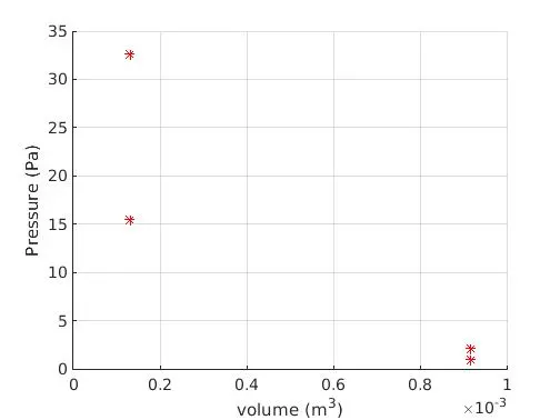
- Now to make the curves, we will have to find the instantabeous pressure and volume values as the piston moves. For that we will define a function piston_kinematics(). this will intake certain inputs to calculate only the instantaneous volume by the help of the equation 5 in the PRE-REQUISITES.
function V =  piston_kinematics(bore,stroke,connecting_rod,cr,start_crank,end_crank)


              % Required Inputs

              a=stroke/2;
              R=connecting_rod/a;

              v_s = (pi/4)*bore^2*stroke;
              v_c = v_s/(cr-1);

              theta = linspace(start_crank,end_crank,100);

              Q1 = (cr-1)*0.5;
              Q2 = R+1-cosd(theta);
              Q3 = (R^2-sind(theta).^2).^0.5;

              V = (1 + Q1*(Q2 - Q3)).*v_c;

         end
- The above function is used in the processess isentropic compression and isentropic expansion the other two processes, are carried out under constant volume (isochoric) process. So these will be defined under state 2 and state 3 values respectively. after getting the instantaneous volume valeue from the function it is used to calulated the instantaneous pressure value for both the states respectively. the code is as shown below.
 % STATE 2 VALUES
V_compression = piston_kinematics(bore,stroke,connecting_rod,cr,180,0);  % from the function, piston_kinematics()
constant_c = p1*v1^gamma;                                                % for calculating the instantaaneous pressure
P_compression = constant_c./V_compression.^gamma;                        % pressure value is obtained
% STATE 3 VALUES
V_expansion = piston_kinematics(bore,stroke,connecting_rod,cr,0,180);    % from the function, piston_kinematics()
constant_c = p3*v3^gamma;                                                % for calculating the instantaaneous pressure
P_expansion = constant_c./V_expansion.^gamma; % pressure value is obtained- Atlast the plotting statements for the curves from 1 →">→→ 2 and 3 →">→→ 4, based on the above statements.
plot(V_compression,P_compression)    % this plots the isentropic curve from state 1 to state 2 (note-state 2 is not included)


plot(V_expansion,P_expansion) % this plots the isentropic curve from state 3 to state 4 (note-state 4 is not included)- Also for the curves from 2→">→→3 and 4→">→→1 are also added to the main coding.
plot([v2 v3],[p2 p3],'color','b')    % this plots the isochoric curve from state 2 to state 3 (note-state 3 is not included)


plot([v4 v1],[p4 p1],'color','b')    % this plots the isochoric curve from state 4 to state 1
- Also find the thermal efficiency.
MAIN PROGRAM
function V =  piston_kinematics(bore,stroke,connecting_rod,cr,start_crank,end_crank)


% Required Inputs

a=stroke/2;
R=connecting_rod/a;

v_s = (pi/4)*bore^2*stroke;
v_c = v_s/(cr-1);

theta = linspace(start_crank,end_crank,100);

Q1 = (cr-1)*0.5;
Q2 = R+1-cosd(theta);
Q3 = (R^2-sind(theta).^2).^0.5;

V = (1 + Q1*(Q2 - Q3)).*v_c;

end
% OTTO CYCLE USING MATLAB
% Required Inputs
% ENGINE PARAMETRES
bore=0.1; % bore diameter (m)
stroke=0.1; % stroke length (m)
connecting_rod=0.15; % connecting rod length (m)
cr=12; % compression ratio
gamma=1.4; % adiabatic constant or specific heat ratio
% STATE 1 PARAMETRES
p1 = 101325; % pressure (Pa) at the start of compression
t1 = 500; % temperature (K) at the start of compression
% CALCULATING SWEPT AND CLEARANCE VOLUME
v_swept = (pi/4)* bore^2 * stroke; % volume (m^3) swept by the piston
v_clearance = v_swept/(cr-1); % clearance volume
v1 = v_swept+v_clearance; % volume at the start of the compression
% STATE 2 VALUES
% p2*v2^gamma = p1*v1^gamma
% (v1/v2)=cr
v2 = v_clearance; % volume at the start of combustion
p2 = p1*cr^gamma; % pressure at the start of combustion
% (p2*v2)/t2 = (p1*v1)/t1
t2 = p2*v2*t1/(p1*v1); % temperature at the start of combustion
V_compression = piston_kinematics(bore,stroke,connecting_rod,cr,180,0); % from the function, piston_kinematics()
constant_c = p1*v1^gamma; % for calculating the instantaaneous pressure
P_compression = constant_c./V_compression.^gamma; % pressure value is obtained
% STATE 3 VALUES
v3 = v2; % volume at the end of the combustion
t3 = 2300; % temperature at the end of the combustion
% (p2/t2) = (p3/t3)
p3 = (p2*t3)/t2; % pressure at the end of the combustion
V_expansion = piston_kinematics(bore,stroke,connecting_rod,cr,0,180); % from the function, piston_kinematics()
constant_c = p3*v3^gamma; % for calculating the instantaaneous pressure
P_expansion = constant_c./V_expansion.^gamma; % pressure value is obtained
% STATE 4 VALUES
v4 = v1; % volume at the end of the power stroke
% p4*v4^gamma = p3*v3^gamma
p4 = p3*(v3/v4)^gamma; % oressure at the end of the power stroke
t4 =(p4*v4*t3)/(p3*v3);
% THERMAL EFFICIENCY
eff = (1-1/cr^(gamma-1))*100
%PLOTTING
figure(1)
hold on
plot(v1,p1,'*','color','red') % this plots only the state 1
plot(V_compression,P_compression) % this plots the isentropic curve from state 1 to state 2 (note-state 2 is not included)
plot(v2,p2,'*','color','blue') % this plots only the state 2
plot([v2 v3],[p2 p3],'color','magenta') % this plots the isochoric curve from state 2 to state 3 (note-state 3 is not included)
plot(v3,p3,'*','color','green') % this plots only the state 3
plot(V_expansion,P_expansion) % this plots the isentropic curve from state 3 to state 4 (note-state 4 is not included)
plot(v4,p4,'*','color','yellow') % this plots only the state 4
plot([v4 v1],[p4 p1],'color','cyan') % this plots the isochoric curve from state 4 to state 1
xlabel('VOLUME (m^3)') % the x axis is labelled as "VOLUME (m^3)"
ylabel('PRESSURE (Pa)') % the y axis is labelled as "PRESSURE (Pa)"
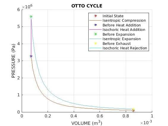
legend("Initial State","Isentropic Compression","Before Heat Addition","Isochoric Heat Addition","Before Expansion","Isentropic Expansion","Before Exhaust","Isochoric Heat Rejection") % For labelling the curves
title("OTTO CYCLE")
grid on
RESULT
- P-V Diagram
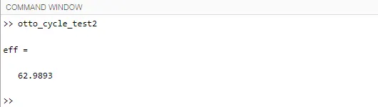
- Command Window
CONCLUSION
- The matlab program is successful compiled
- The P-V diagram for the otto cycle was successfully plotted
- The thermal efficiency is 62.9893%
- The efficiency depends on compression ratio.But at higher compression ratio, knocking can occur, therefore, an optimum compressio ratio must be preffered.
- The error occured is attached as a document file.