GENETIC ALGORITHM USING MATLAB
AIM.
Understanding Genetic Algorithm (GA)
OBJECTIVES
- Explain the concept of genetic algorithm in your own words and also explain the syntax for ga in MATLAB in your report.
- Write a code in MATLAB to optimise the stalagmite function and find the global maxima of the function.
- Plot graphs for all 3 studies and for F maximum vs no. of iterations.
PRE-REQUISITES
Before getting into the GA, we have to know its origin.
What is an algorithm ? algorithm is a finite sequence of well defined, computer-implementable instructions, typically to solve a class of problems or to perform a computation.
What is optimization ? Optimising means finding the best solution from all feasible solutions. It is the maximizing or minimizing a real function by systematically choosing input values from within an allowed set and computing the value of the function.
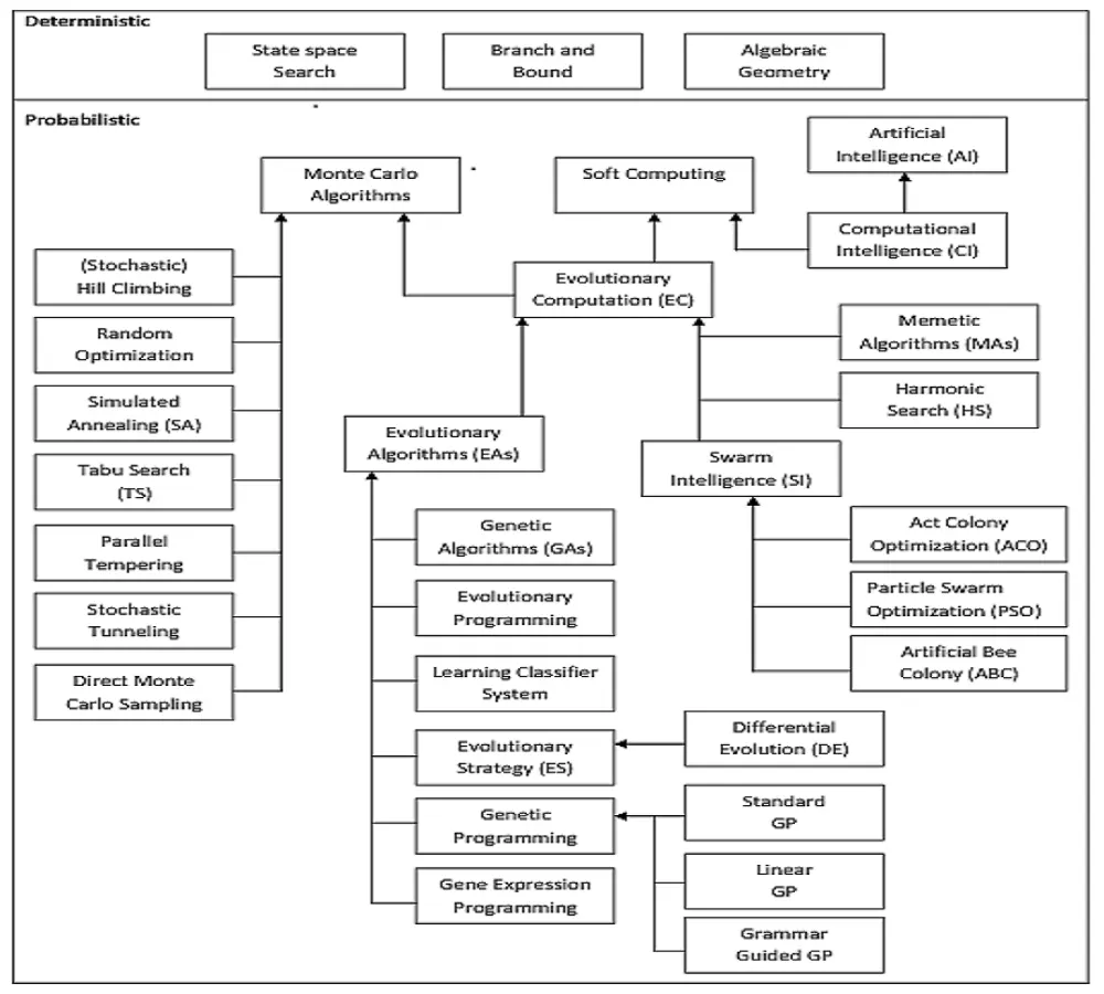
Here we are particularly interested in mathematical optimization, i.e. the selection of a best element from some set of available alternatives by means of applied mathematics. the below mention taxonamy can be referred for better understanding.
OBJECTIVE-1
What Is the Genetic Algorithm?
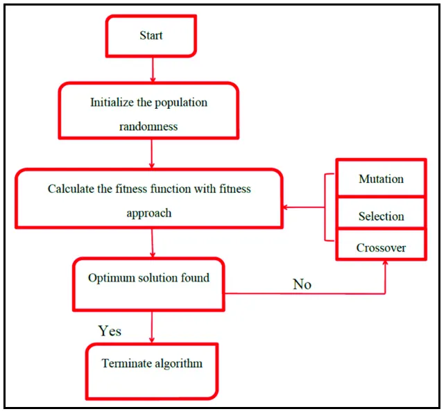
- The genetic algorithm is a method for solving optimization problems that is based on natural selection, the process that drives biological evolution.
- It repeatedly modifies a population of individual solutions.
- At each step, the genetic algorithm selects individuals at random from the current population to be parents and uses them produce the children for the next generation.
- Over successive generations, the population “evolves” toward an optimal solution.
Governing Rules of Genetic Algorithm:- The genetic algorithm uses three main types of rules at each step to create the next generation from the current population:
•Selection rules select the individuals, called parents, that contribute to the population at the next generation.
•Crossover rules combine two parents to form children for the next generation.
•Mutation rules apply random changes to individual parents to form children.
STANDARD VS GENETIC ALGORITHM
| Standard Algorithm | Genetic Algorithm |
| Generates a single point at each iteration. The sequence of points approaches an optimal solution. |
Generates a population of points at each iterations. The population approaches an optimal solutions. |
| Selects the next point in the sequence by a deterministic computation. | Selects the next population by computations that involve random choices. |
How to use the Genetic Algorithm?
There are two ways you can use the genetic algorithm:-
•Calling the genetic algorithm function ga at the command line.
Syntax `to` 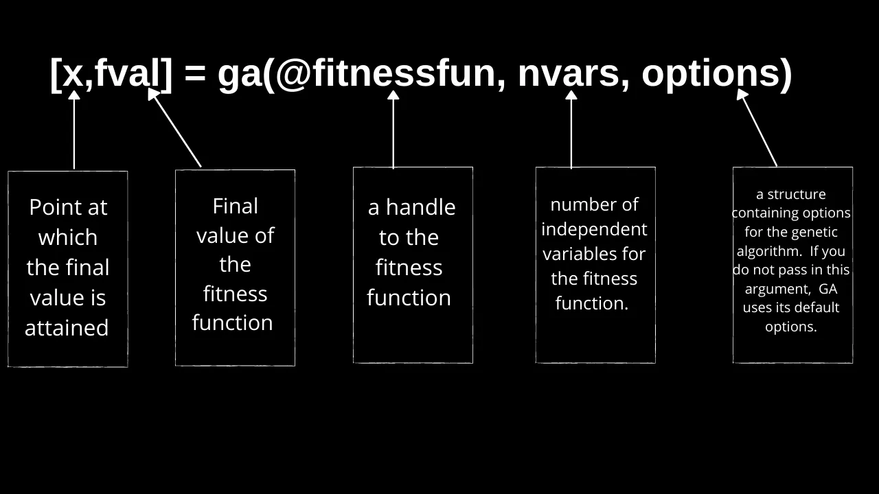
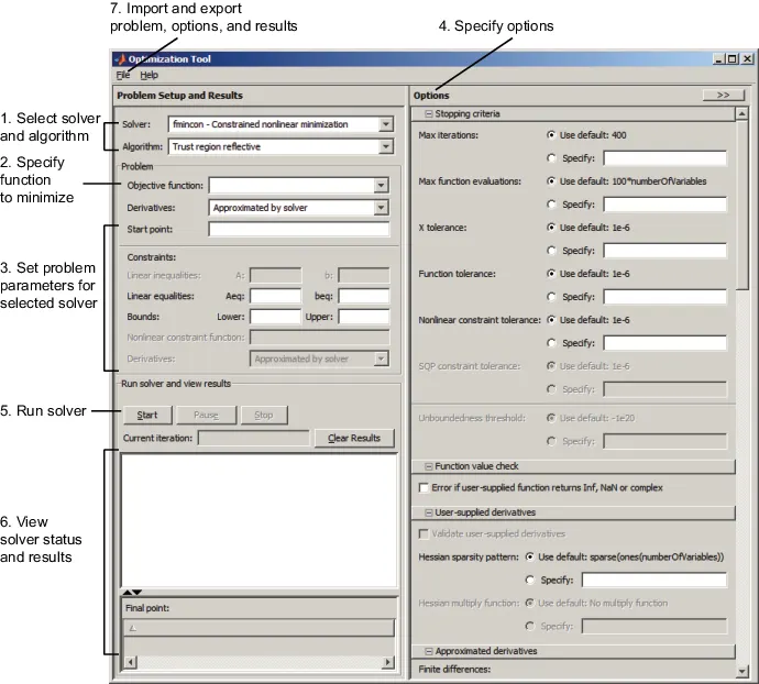
•Using the Genetic Algorithm Tool, a graphical interface to the genetic algorithm.
Maximizing Vs Minimizing
- The optimization functions in the Genetic Algorithm minimize the objective or fitness function.That is, they solve problems of the form :- `min f(x)`
- If you want to maximize f(x), you can do so by minimizing -f(x), because the point at which the minimum of -f(x) occurs is the same as the point at which the maximum of f(x) occurs.
OBJECTIVE - 2
PROCEDURE
- The first step is to define the search limit. The GA algorithm requires a set of imaginary space to run down its algorithm. Here we define the limits of x and y coordinates in an array format. So that combination of (x,y) coordinates will deliver a sample for GA to work with. Also the GA algorithm doesn't know that it can go beyond the defined x and y coordinaes.
x = linspace(0,0.6,150);                       % X-axis search limit for GA algorithm
y = linspace(0,0.6,150); % Y-axis search limit for GA algorithm - Now we need a search space to analyse the plots that we will be creating. Since we have the search limits from the above step. Using that we will create 2d coordinates that forms a grid. This grid space can used to evaluate the stalgamite function by plotting the required coordinates. This grid is formed using the inbuilt MATLAB function meshgrid(). In the code below, xx and yy are both 150x150 matrix.
[xx,yy] = meshgrid(x,y); % this creates a 2d coordinate grid or mesh
- Now we will define the stalagmite function that includes all the mathematical expressions to define the stalagmite growth.
% STALAGMITE FUNCTION DEFINITION


function [f1] = stalagmite(input)                       % function is defined with a row vector 'input'

    x1 = input(1);                                      % assigning the first element of 'input' vector to x1
    y1 = input(2);                                      % assigning the second element of 'input' vector to x1

    f1_x = (sin(5.1*pi*x1+0.5))^6;                      %
    f1_y = (sin(5.1*pi*y1+0.5))^6;                      %
    f2_x = exp(-4*log(2)*(x1-0.0667)^2/0.64);           % lines from 9 to 14 defines the required mathematical
    f2_y = exp(-4*log(2)*(y1-0.0667)^2/0.64);           % expressions to define the stalagmite function

    f1 = -(f1_x * f1_y * f2_x * f2_y);                  %

end % function ends- Then we have to call this "stalagmite" function. it is done inside a nesting 'for' loop. Because we need to find the golbal maximum of the function in the grid that we have defined. So to access that grid we need nesting for loops. This grid is nothing made from 2 square matrices, designed to accomodate the x and y axis coordinates, respectively. we will define the (x,y) coordinates in such a way that there is 150 combinations of 1 x-coordinate alone with all the y- coordinates. Therefore, we have a total grid points of 22500 (i.e 150*150). The statements inside the nested for loop is commented in the code itself.
% EVALUATING THE STALGAMITE FUNCTION
    for i=1:length(xx)                         % gives indexing for the x-coordinates
    for j=1:length(yy)                         % gives indexing for the y-coordinates
        input_vector(1) = xx(i,j);             % the corresponding element square matrix 'xx' is assigned to the 'input_vector'
        input_vector(2) = yy(i,j);             % the corresponding element square matrix 'yy' is assigned to the 'input_vector'
        f(i,j) = stalagmite(input_vector);     % stalgamite function is called
    end                                        % nested for loop ends
end % outside for loop ends- Now we will plot the 3d surface using surfc(). It requires 3 inputs- square matrices xx & yy and the stalagmite function output. Also the 3d plot is given a good shading colors by means of the statement 'shading interp'. It varies the color in each line segment and face by interpolating the colormap index or true color value across the line or face.
% CREATING 3D SURFACE OF THE STALAGMITE FUNCTION
surfc(xx,yy,f)                                        % creates 3d surface with the 2d square matrices xx & yy, along with the function output
xlabel('X- value')                                    % labelling the x-axis
ylabel('Y- value')                                    % labelling the y-axis
shading interp                                        % provides proper shading to the 3d surfaces
- Now the GA algorithm is called using the function handle '@stalagmite' along wit 2 inputs- x and y. Its gives 2 outputs. one is the row vector giving coordinates of minimized stalagmite function (i.e. inputs(1) & inputs(2)). Second is the minimized stalagmite function value (i.e. fval).
% RUNNING THE GA ALGORITHM
[inputs,fval] = ga(@stalagmite,2)                     % GA function is called
NOTE:- Go throuh the below program which is the compliation of above described steps:-
% STALAGMITE FUNCTION DEFINITION


function [f1] = stalagmite(input)                       % function is defined with a row vector 'input'

    x1 = input(1);                                      % assigning the first element of 'input' vector to x1
    y1 = input(2);                                      % assigning the second element of 'input' vector to x1

    f1_x = (sin(5.1*pi*x1+0.5))^6;                      %
    f1_y = (sin(5.1*pi*y1+0.5))^6;                      %
    f2_x = exp(-4*log(2)*(x1-0.0667)^2/0.64);           % lines from 9 to 14 defines the required mathematical
    f2_y = exp(-4*log(2)*(y1-0.0667)^2/0.64);           % expressions to define the stalagmite function

    f1 = (f1_x * f1_y * f2_x * f2_y);                  %

end                                                     % function ends
% MATLAB PROGRAM TO OPTIMIZE STALGAMITE FUNCTION USING GA ALGORITHM
% CLEARING PRE-STORED MEMORY
clear all
clc
% SEARCH LIMITS
x = linspace(0,0.6,150); % X-axis search limit for GA algorithm
y = linspace(0,0.6,150); % Y-axis search limit for GA algorithm
% CREATING A 2D MESH/GRID
[xx,yy] = meshgrid(x,y); % this creates a 2d coordinate grid or mesh
% EVALUATING THE STALGAMITE FUNCTION
for i=1:length(xx) % gives indexing for the x-coordinates
for j=1:length(yy) % gives indexing for the y-coordinates
input_vector(1) = xx(i,j); % the corresponding element square matrix 'xx' is assigned to the 'input_vector'
input_vector(2) = yy(i,j); % the corresponding element square matrix 'yy' is assigned to the 'input_vector'
f(i,j) = stalagmite(input_vector); % stalgamite function is called
end % nested for loop ends
end % outside for loop ends
% CREATING 3D SURFACE OF THE STALAGMITE FUNCTION
surfc(xx,yy,f) % creates 3d surface with the 2d square matrices xx & yy, along with the function output
xlabel('X- value') % labelling the x-axis
ylabel('Y- value') % labelling the y-axis
shading interp % provides proper shading to the 3d surfaces
% RUNNING THE GA ALGORITHM
[inputs,fval] = ga(@stalagmite,2) % GA function is called
OUTPUT:- COMMAND WINDOW AND THE PLOT (upright peaks)
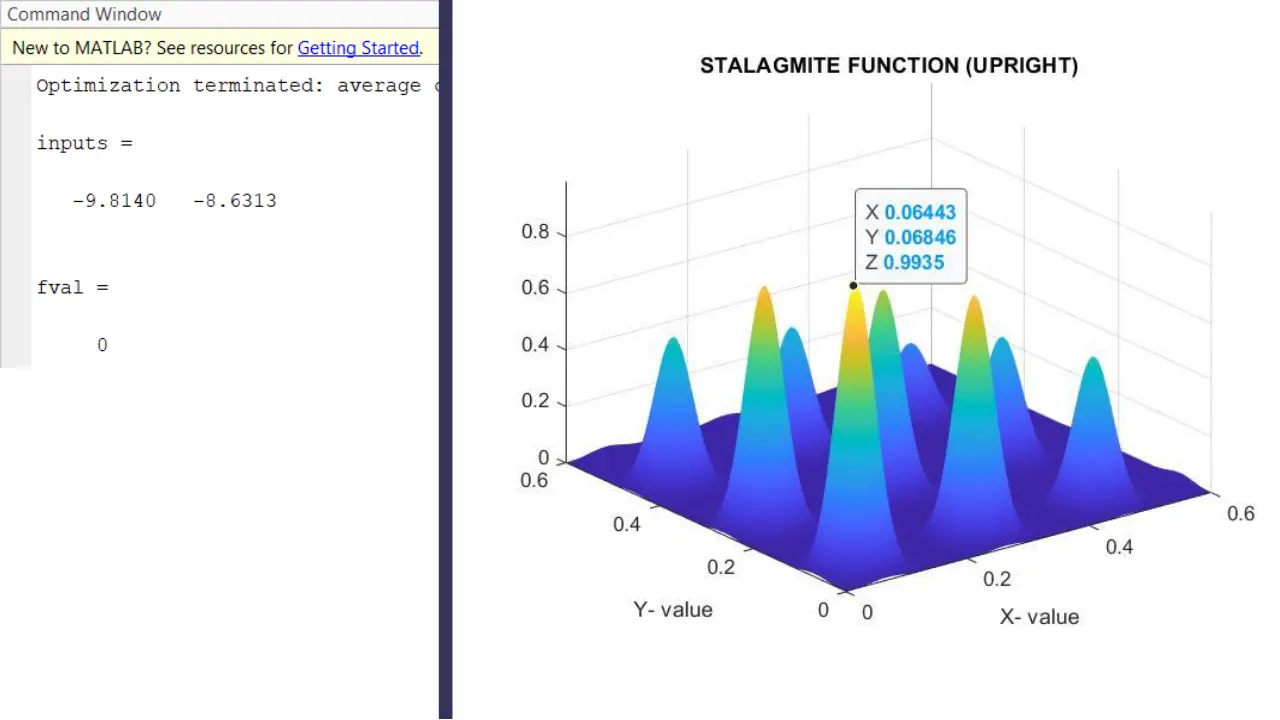
NOTE:- The GA function is used to find the global minimum of stalagmite function value. You can see the above 3d figure is the result of minizing the stalagmite function (i.e. not the upright peaks). But here we want the maximum. So to get the global maximum of stalgamite function value and its coordinates, we will put a (-ve) sign in the output of the stalagmite function. Then the output will be:-
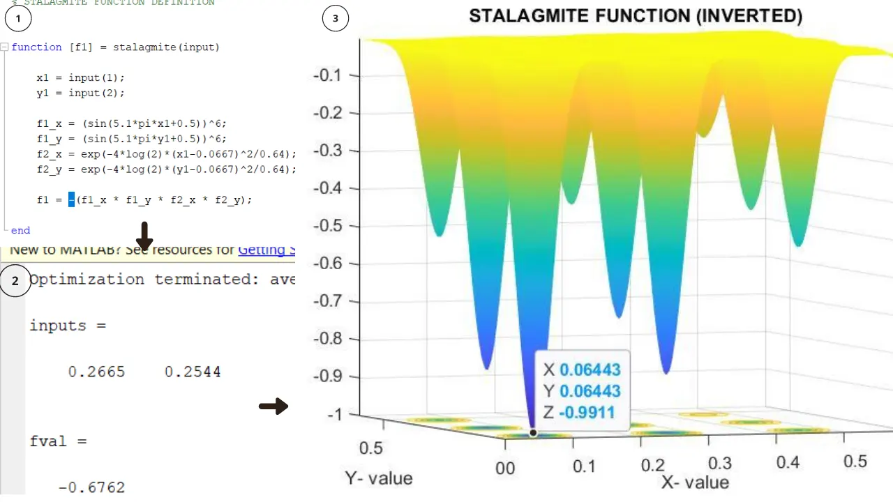
NOTE:- We can see from the above figure that the fval is not 0 and the plot got inverted (i.e. before putting the (-ve) sign the peaks were above 0 and extending between 0 and 1, but after putting the (-ve) sign the peaks are below and extending between 0 and -1).
Hence it became the maximised stalgamite function. But on repeated compiling the program we see the value of fval and inputs keep on changing. Hence we are not getting a consistency and inaccuracy in the output. Then comes the requirement to make some detailed studies.
STUDY-1 - (UNBOUNDED)
Here we defined the number of iterations that GA function will undergo as 50. Then for the study purpose, once again, the stalagmite function is run under the for loop for 50 no:s of iterations. Then the outputs like the X and Y coordinates are stored in the row vector "inp" and the function value of each iterations in the array "fopt". Also the GA algorithms running time is known from tic and toc commands.
For knowing whether we are in the right way, we will plot the outputs in the same figure window by means of subplot command. The subplot-1 will show the 3d stalagmite function using the "surfc()", with unbounded points marked using the plot3 command. The subplot-2 will show the variation of stalagmite function value of each iteration as a function of iterations. The codes are as shown below.
% SUDY 1 - RUNNING THE GA ALGORITHM (UNBOUNDED)
tic                                                   % starting point of the timer
for i=1:iterations                                    % for loop starts for 50 number's of iterations
    [inp,fopt(i)]  = ga(@stalagmite,2);               % GA function is called with "inp" taking the coordinates of each iterations coordinate values and fopt taking the stalagmite function value
    xopt(i) = inp(1);                                 % the x-coordinate of each iteration is assigned to first element of row vector "inp"
    yopt(i) = inp(2);                                 % the y-coordinate of each iteration is assigned to second element of row vector "inp"
end                                                   % for loop ends
time2 = toc                                           % timer stops and the value is assigned to the VARIABLE "TIME2"

figure(2)                                                                        % anew figure window is created
subplot(2,1,1)                                                                   % subplot(m,n,p) divides the current figure into an m-by-n grid and creates axes in the position specified by p
hold on                                                                          % enables overwritting on the first subplot
surfc(x,y,f)                                                                     % creates a 3d surface
shading interp                                                                   % provides proper shading to the 3d surfaces
plot3(xopt,yopt,fopt,'marker','o','markersize',3,'markerfacecolor','b')          % plot3(X,Y,Z,LineSpec) creates the plot using the specified line style, marker, and color.
title('UNBOUNDED POINTS')                                                        % enables title for the subplot-1

subplot(2,1,2)                                                                   % subplot-2 is created below the sunplot-1
plot(fopt)                                                                       % the STALAGMITE optimal function value for each iterations is plotted as a function of iterations (x-axis=iterations,y-axis=fopt)
xlabel('Iterations')                                                             % labels the x-axis as "iterations"
ylabel('STALAGMITE FUNCTION,(fopt)')                                                    % labels the y-axis as the "function value"
title('UNBOUNDED')                                                               % enables title for the subplot-2
OUTPUT:- PLOT
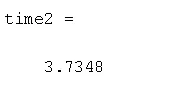 `to` Time taken to complete the Unbounded GA Algorithm
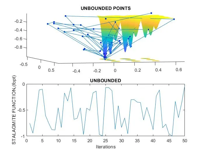
NOTE:- From the above 3d plot, you can see that the points in the subplot-1 is unbounded. The points are all over the place.This is because we are having random sampling and due to this every time i run the program, i get diiferent results. Iin the subplot-2 also, the function value is varying between 0 and -1, which is not a viable solution for our problem. Hence, now also, the stalagmite function coordinates and value will keep on changing. In the study-2 we will define the function within the bounde points.
STUDY-2 - (BOUNDED)
Here we will contain the x and y points within the lower and upper bounds. you would have noticed in the study-1 that the x and y values are going below 0 and above 0.6. We want them to be between 0 & 1 or to be more specific, can be contained within small range also.
For that the function definition of GA is modified:-
Syntax `to`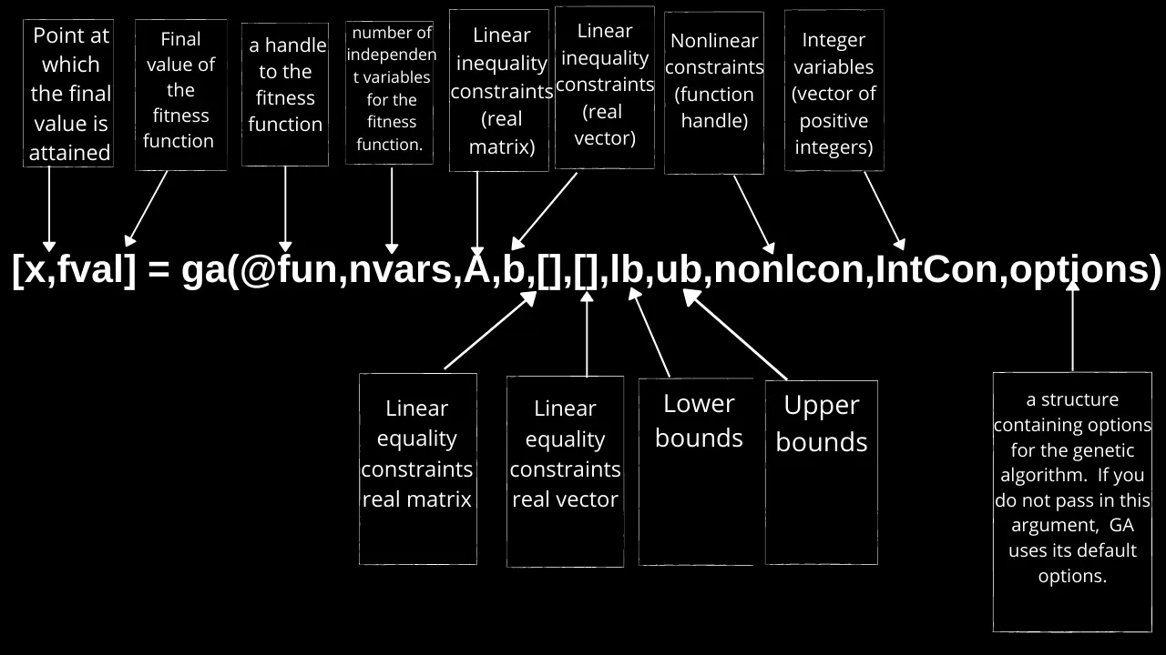
The code is as shown below for study-2:-
% SUDY 2 - RUNNING THE GA ALGORITHM (BOUNDED)
tic                                                                              % starting point of the timer
for j=1:iterations                                                               % for loop starts for 50 number's of iterations
    [inp2,fopt2(j)]  = ga(@stalagmite,2,[],[],[],[],[0;0],[0.6;0.6]);            % GA function is called with "inp" taking the coordinates of each iterations coordinate values and fopt taking the stalagmite function value
    xopt2(j) = inp2(1);                                                          % the x-coordinate of each iteration is assigned to first element of row vector "inp"
    yopt2(j) = inp2(2);                                                          % the y-coordinate of each iteration is assigned to second element of row vector "inp"
end                                                                              % for loop ends
time2 = toc;                                                                     % timer stops and the value is assigned to the VARIABLE "TIME2"

figure(3)                                                                        % anew figure window is created
subplot(2,1,1)                                                                   % subplot(m,n,p) divides the current figure into an m-by-n grid and creates axes in the position specified by p
hold on                                                                          % enables overwritting on the first subplot
surfc(x,y,f)                                                                     % creates a 3d surface
shading interp                                                                   % provides proper shading to the 3d surfaces
plot3(xopt2,yopt2,fopt2,'marker','o','markersize',5,'markerfacecolor','b')       % plot3(X,Y,Z,LineSpec) creates the plot using the specified line style, marker, and color.
title('BOUNDED POINTS')                                                          % enables title for the subplot-1

subplot(2,1,2)                                                                   % subplot-2 is created below the sunplot-1
plot(fopt2)                                                                      % the STALAGMITE optimal function value for each iterations is plotted as a function of iterations (x-axis=iterations,y-axis=fopt)
xlabel('Iterations')                                                             % labels the x-axis as "iterations"
ylabel('STALAGMITE FUNCTION,(fopt2)')                                            % labels the y-axis as the "function value"
title('BOUNDED')                                                                 % enables title for the subplot-2

fprintf('%sn','STUDY-2')
fprintf('The number of iterations is 50n')
fprintf('The time taken for study-2 is:%fn',time2)
fprintf('The X & Y coordinates are: %f %fn',inp2(1),inp2(2))
fprintf('The global maximum of stalagmite function is %fn',mean(fopt2))
OUTPUT:- COMMAND WINDOW & PLOT
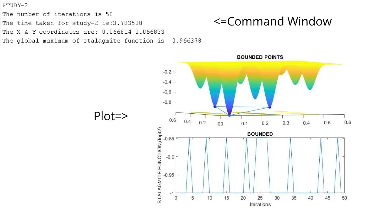
NOTE:- Here the plot is better than that of study-1. We can make the variations of subplot-2 of above figure more accurate in the study-3.
STUDY - 3 - (INCREASING THE POPULATION)
Here the code by means of population "options". Population options let you specify the parameters of the population that the genetic algorithm uses. It is given by:-
options = optimoptions(solvername), where the solvername is ga
options = optimoptions(oldoptions,name,value), where oldoptions = options, name = population size and the value has to be increased to 170, because in study-2 & study-3, the options in the ga function where default. Then the population is defaultly calculated at 50. For now we are making it 170, as the options are manually defined. The code is as follows:-
% SUDY-3 - RUNNING THE GA ALGORITHM (POPULATION IS INCREASED)
options = optimoptions('ga');
options = optimoptions(options,'PopulationSize',170);
Iterations = 100;

tic                                                                                           % starting point of the timer
for k=1:Iterations                                                                            % for loop starts for 50 number's of iterations
    [inp3,fopt3(k)]  = ga(@stalagmite,2,[],[],[],[],[0;0],[0.6;0.6],[],[],options);           % GA function is called with "inp" taking the coordinates of each iterations coordinate values and fopt taking the stalagmite function value
    xopt3(k) = inp3(1);                                                                       % the x-coordinate of each iteration is assigned to first element of row vector "inp"
    yopt3(k) = inp3(2);                                                                       % the y-coordinate of each iteration is assigned to second element of row vector "inp"
end                                                                                           % for loop ends
time3 = toc                                                                                   % timer stops and the value is assigned to the VARIABLE "TIME2"

figure(4)                                                                        % anew figure window is created
subplot(2,1,1)                                                                   % subplot(m,n,p) divides the current figure into an m-by-n grid and creates axes in the position specified by p
hold on                                                                          % enables overwritting on the first subplot
surfc(x,y,f)                                                                     % creates a 3d surface
shading interp                                                                   % provides proper shading to the 3d surfaces
plot3(xopt3,yopt3,fopt3,'marker','o','markersize',5,'markerfacecolor','b')       % plot3(X,Y,Z,LineSpec) creates the plot using the specified line style, marker, and color.
title('BOUNDED POINTS')                                                          % enables title for the subplot-1

subplot(2,1,2)                                                                   % subplot-2 is created below the sunplot-1
plot(fopt3)                                                                      % the STALAGMITE optimal function value for each iterations is plotted as a function of iterations (x-axis=iterations,y-axis=fopt)
xlabel('Iterations')                                                             % labels the x-axis as "iterations"
ylabel('STALAGMITE FUNCTION,(fopt3)')                                            % labels the y-axis as the "function value"
title('BOUNDED')                                                                 % enables title for the subplot-2

fprintf('STUDY-3n')
fprintf('The number of iterations is 100n')
fprintf('The time taken for study-3 is:%fn',time3)
fprintf('The X & Y coordinates are: %f %fn',inp3(1),inp3(2))
fprintf('The global maximum of stalagmite function is %fn',mean(fopt3))

Total_Study = time+time1+time2+time3;
fprintf('The total time taken for whole study is:%fn',Total_Study)
OUTPUT:- COMMAND WINDOW & PLOTS
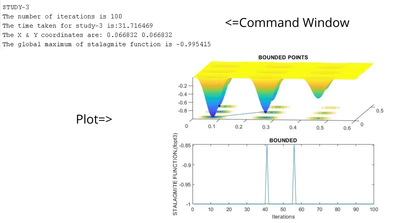 NOTE:- Now you see the maximum variations have been reduced. On repeated compiling of the program, we get slight variations in output. And to neglect them we again contain the LB and UB or by increasing the population size.
WHOLE PROGRAM AND OUTPUT
% STALAGMITE FUNCTION DEFINITION


function [f1] = stalagmite(input)                       % function is defined with a row vector 'input'

    x1 = input(1);                                      % assigning the first element of 'input' vector to x1
    y1 = input(2);                                      % assigning the second element of 'input' vector to x1

    f1_x = (sin(5.1*pi*x1+0.5))^6;                      %
    f1_y = (sin(5.1*pi*y1+0.5))^6;                      %
    f2_x = exp(-4*log(2)*(x1-0.0667)^2/0.64);           % lines from 9 to 14 defines the required mathematical
    f2_y = exp(-4*log(2)*(y1-0.0667)^2/0.64);           % expressions to define the stalagmite function

    f1 = -(f1_x * f1_y * f2_x * f2_y);                  %

end                                                     % function ends
% MATLAB PROGRAM TO OPTIMIZE STALGAMITE FUNCTION USING GA ALGORITHM
% CLEARING PRE-STORED MEMORY
clear all
close all
clc
% SEARCH LIMITS
x = linspace(0,0.6,150); % X-axis search limit for GA algorithm
y = linspace(0,0.6,150); % Y-axis search limit for GA algorithm
% CREATING A 2D MESH/GRID
[xx,yy] = meshgrid(x,y); % this creates a 2d coordinate grid or mesh
iterations = 50; % number of iterations for GA functions
% EVALUATING THE STALGAMITE FUNCTION
tic
for i=1:length(xx) % gives indexing for the x-coordinates
for j=1:length(yy) % gives indexing for the y-coordinates
input_vector(1) = xx(i,j); % the corresponding element square matrix 'xx' is assigned to the 'input_vector'
input_vector(2) = yy(i,j); % the corresponding element square matrix 'yy' is assigned to the 'input_vector'
f(i,j) = stalagmite(input_vector); % stalgamite function is called
end % nested for loop ends
end % outside for loop ends
time = toc;
% CREATING 3D SURFACE OF THE STALAGMITE FUNCTION
figure(1)
surfc(xx,yy,f) % creates 3d surface with the 2d square matrices xx & yy, along with the function output
xlabel('X- value') % labelling the x-axis
ylabel('Y- value') % labelling the y-axis
shading interp % provides proper shading to the 3d surfaces
fprintf('%sn','FIRST COMPILATION WITHOUT STUDY')
fprintf('The number of iterations is 150n')
fprintf('The time taken is:%fn',time)
fprintf('The X & Y coordinates are: %f %fn',input_vector(1),input_vector(2))
fprintf('The global maximum of stalagmite function is %fn',mean(f))
% SUDY 1 - RUNNING THE GA ALGORITHM (UNBOUNDED)
tic % starting point of the timer
for i=1:iterations % for loop starts for 50 number's of iterations
[inp1,fopt1(i)] = ga(@stalagmite,2); % GA function is called with "inp" taking the coordinates of each iterations coordinate values and fopt taking the stalagmite function value
xopt1(i) = inp1(1); % the x-coordinate of each iteration is assigned to first element of row vector "inp"
yopt1(i) = inp1(2); % the y-coordinate of each iteration is assigned to second element of row vector "inp"
end % for loop ends
time1 = toc; % timer stops and the value is assigned to the VARIABLE "TIME2"
figure(2) % anew figure window is created
subplot(2,1,1) % subplot(m,n,p) divides the current figure into an m-by-n grid and creates axes in the position specified by p
hold on % enables overwritting on the first subplot
surfc(x,y,f) % creates a 3d surface
shading interp % provides proper shading to the 3d surfaces
plot3(xopt1,yopt1,fopt1,'marker','o','markersize',3,'markerfacecolor','b') % plot3(X,Y,Z,LineSpec) creates the plot using the specified line style, marker, and color.
title('UNBOUNDED POINTS') % enables title for the subplot-1
subplot(2,1,2) % subplot-2 is created below the sunplot-1
plot(fopt1) % the STALAGMITE optimal function value for each iterations is plotted as a function of iterations (x-axis=iterations,y-axis=fopt)
xlabel('Iterations') % labels the x-axis as "iterations"
ylabel('STALAGMITE FUNCTION,(fopt1)') % labels the y-axis as the "function value"
title('UNBOUNDED') % enables title for the subplot-2
fprintf('%sn','STUDY-1')
fprintf('The number of iterations is 50n')
fprintf('The time taken for study-1 is:%fn',time1)
fprintf('The X & Y coordinates are: %f %fn',inp1(1),inp1(2))
fprintf('The global maximum of stalagmite function is %fn',mean(fopt1))
% SUDY 2 - RUNNING THE GA ALGORITHM (BOUNDED)
iterations=50;
tic % starting point of the timer
for j=1:iterations % for loop starts for 50 number's of iterations
[inp2,fopt2(j)] = ga(@stalagmite,2,[],[],[],[],[0;0],[0.6;0.6]); % GA function is called with "inp" taking the coordinates of each iterations coordinate values and fopt taking the stalagmite function value
xopt2(j) = inp2(1); % the x-coordinate of each iteration is assigned to first element of row vector "inp"
yopt2(j) = inp2(2); % the y-coordinate of each iteration is assigned to second element of row vector "inp"
end % for loop ends
time2 = toc; % timer stops and the value is assigned to the VARIABLE "TIME2"
figure(3) % anew figure window is created
subplot(2,1,1) % subplot(m,n,p) divides the current figure into an m-by-n grid and creates axes in the position specified by p
hold on % enables overwritting on the first subplot
surfc(x,y,f) % creates a 3d surface
shading interp % provides proper shading to the 3d surfaces
plot3(xopt2,yopt2,fopt2,'marker','o','markersize',5,'markerfacecolor','b') % plot3(X,Y,Z,LineSpec) creates the plot using the specified line style, marker, and color.
title('BOUNDED POINTS') % enables title for the subplot-1
subplot(2,1,2) % subplot-2 is created below the sunplot-1
plot(fopt2) % the STALAGMITE optimal function value for each iterations is plotted as a function of iterations (x-axis=iterations,y-axis=fopt)
xlabel('Iterations') % labels the x-axis as "iterations"
ylabel('STALAGMITE FUNCTION,(fopt2)') % labels the y-axis as the "function value"
title('BOUNDED') % enables title for the subplot-2
fprintf('%sn','STUDY-2')
fprintf('The number of iterations is 50n')
fprintf('The time taken for study-2 is:%fn',time2)
fprintf('The X & Y coordinates are: %f %fn',inp2(1),inp2(2))
fprintf('The global maximum of stalagmite function is %fn',mean(fopt2))
% SUDY-3 - RUNNING THE GA ALGORITHM (POPULATION IS INCREASED)
options = optimoptions('ga');
options = optimoptions(options,'PopulationSize',170);
Iterations = 100;
tic % starting point of the timer
for k=1:Iterations % for loop starts for 50 number's of iterations
[inp3,fopt3(k)] = ga(@stalagmite,2,[],[],[],[],[0;0],[0.6;0.6],[],[],options); % GA function is called with "inp" taking the coordinates of each iterations coordinate values and fopt taking the stalagmite function value
xopt3(k) = inp3(1); % the x-coordinate of each iteration is assigned to first element of row vector "inp"
yopt3(k) = inp3(2); % the y-coordinate of each iteration is assigned to second element of row vector "inp"
end % for loop ends
time3 = toc % timer stops and the value is assigned to the VARIABLE "TIME2"
figure(4) % anew figure window is created
subplot(2,1,1) % subplot(m,n,p) divides the current figure into an m-by-n grid and creates axes in the position specified by p
hold on % enables overwritting on the first subplot
surfc(x,y,f) % creates a 3d surface
shading interp % provides proper shading to the 3d surfaces
plot3(xopt3,yopt3,fopt3,'marker','o','markersize',5,'markerfacecolor','b') % plot3(X,Y,Z,LineSpec) creates the plot using the specified line style, marker, and color.
title('BOUNDED POINTS') % enables title for the subplot-1
subplot(2,1,2) % subplot-2 is created below the sunplot-1
plot(fopt3) % the STALAGMITE optimal function value for each iterations is plotted as a function of iterations (x-axis=iterations,y-axis=fopt)
xlabel('Iterations') % labels the x-axis as "iterations"
ylabel('STALAGMITE FUNCTION,(fopt3)') % labels the y-axis as the "function value"
title('BOUNDED') % enables title for the subplot-2
fprintf('STUDY-3n')
fprintf('The number of iterations is 100n')
fprintf('The time taken for study-3 is:%fn',time3)
fprintf('The X & Y coordinates are: %f %fn',inp3(1),inp3(2))
fprintf('The global maximum of stalagmite function is %fn',mean(fopt3))
Total_Study = time+time1+time2+time3;
fprintf('The total time taken for whole study is:%fn',Total_Study)
OUTPUT:- PLOTS & THE COMMAND WINDOW
- For Study-1
- For Study-2
- For Study-3
RESULT
- The Genetic Algorithm and its syntax is explained properly
- The MATLAB code for Stalagmite function is carried out using GA in MATLAB
- The statistical studies are carried out and corresponding outputs are plotted in graph.
- The GA function outputs are not constant but they will continously change till the optimal solution is obtained.We can stop when the error in the outputs is infinitesimally small.
REFERENCES
http://cda.psych.uiuc.edu/matlab_pdf/gads_tb.pdf
https://arxiv.org/ftp/arxiv/papers/1308/1308.4675.pdf
https://skill-lync.freshdesk.com/support/solutions/articles/43000584189-genetic-algorithm-explained-