WIDE OPEN THROTTLE (WOT)
AIM
Implementing the Wide Open Throttle (WOT)
OBJECTIVE-1 `to`What is the ratio of hill-climbing power required by fully loaded tata ultra truck to the half-loaded one?
OBJECTIVE-2 `to`A flyover is planned to be constructed on a national highway. Keeping in mind about the gradeability for trucks, how much can be the minimum length of the flyover, considering the minimum height at the summit should be 5.5 meters? State your assumptions.
OBJECTIVE-3 `to`Refer to below link for vehicle modelling using Simulink:
Prepare a new drive cycle excel file for the model and also include a hill-climbing angle to it. Revise the model file “Driver_Glider.slx” and comment on the results
OBJECTIVE-4 `to`Model the WOT (Wide Open Throttle) response of GM EV1 car. Compare it with the official figures of the performance of a real vehicle. Prepare a table showing variation in acceleration time with a 5% change in vehicle parameters.
PRE-REQUISITES
What is a Traction Force?`implies`the force propelling the vehicle forward, transmitted to the ground through the drive wheels. The force propelling the vehicle forward, the tractive effort, has to accomplish
the following:
• overcome the rolling resistance;
• overcome the aerodynamic drag;
• provide the force needed to overcome the component of the vehicle’s weight acting
down the slope;
• accelerate the vehicle, if the velocity is not constant.
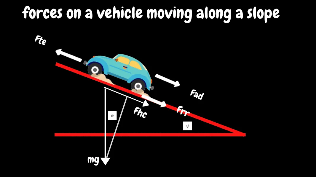
Hill Climbing Force (`Funderset(hc)()`)`to`The force needed to drive the vehicle up a slope. It is simply the component of the vehicle weight that acts along the slope.The equation is:-
`Funderset(hc)()=mgsin(psi)`
OBJECTIVE-1 `implies`What is the ratio of hill-climbing power required by fully loaded tata ultra truck to the half-loaded one?
The Tata Ultra is a LCV (Luggage Carrying Vehicle) from the Tata motors. The Tata Ultra offers maximum permissible GVW in its category of 10400kg and a kerb weight of just 3620kg means it offers the best in the class payload of 7280kg.
NOTE:- Here i have taken the fullyloaded weight is the sum of kerb and paload weight, whereas the half loaded weight is sum of kerb and half of payload weight.
Fully- loaded weight = 3620Kg + 7280Kg Half-loaded weight = 3620Kg + 3640Kg
=10900Kg =7260Kg
The excel sheet with the required ratio output of fully-loaded power to the half-loaded power:-

Ratio is 1.50137741
Google drive link for the excel sheets:-
https://drive.google.com/file/d/1GOKb6RQOv9wDENkI0m98MQ5iiGRNJ0Rt/view?usp=sharing
OBJECTIVE-2
A flyover is planned to be constructed on a national highway. Keeping in mind about the gradeability for trucks, how much can be the minimum length of the flyover, considering the minimum height at the summit should be 5.5 meters? State your assumptions.
What is Gradeability? Gradeability by definition is the ability of a vehicle to negotiate a grade/slope/acclivity in Gross Vehicle Weight (GVW) condition and it can vary from 0 to 45% (maximum).
How is it calculated? Suppose you are running over a slope. You have covered 100m horizontal distance over that slope and climbed a height of 30m. This way, your vehicle is having a gradability of 30%(ie.`30/100*100 %`)
But, that is not maximum. Maximum can be calculated or judged by driving your vehicle on different slopes in increasing slope height manner. The maximum slope that your vehicle can easily climb without shuddering will be the maximum gradability of your vehicle. Or instead you can keep the grade slope same and can change the vehicle’s pay load (or weight on the vehicle) to find the maximum gradability of your vehicle. This is can then be calculated through unitary method – (This is the way gradability is calculated in the world of automobile by Test Engineers).
How is Gradeability for a truck? Now, as we all know that we don’t have 100% flat roads for transportation, we must have a transportation medium that can climb every slope in its way. And it is vehicle manufacturer’s responsibility to make their product suitable for the market. In simplest terms, off-road gradeability in the steepest hill, a truck can climb when running at peak engine torque in its lowest transmission gear
ASSUMPTIONS
For example, a truck climbing a sloppy road with a 12% grade (i.e. rising 12 feet vertically in 100 linear feet) would need 12-percent gradeability to reach the top. And, for every inch the truck's tires penetrate into soft ground, an additional 6 percent gradeability is required. So, if the truck's tires sink 3 inches into loose gravel on the 12-percent grade, then the truck would need 30% gradeability (i.e. 12 + 18) to get up the hill.
But what if the sloppy road momentarily stops the truck on the grade? The average truck with a manual transmission needs around 10 percent gradeability just to get moving from a dead stop. Our example truck, then, better have at least 40% gradeability (i.e. 10 + 12 + 18), or rolling backward down the hill may be the only option.
The following formula calculates gradeability (G) for automobiles. You need to know tractive effort (TE) and gross weight (GW),
`G (%) = 100 *(TE)/(GW)`
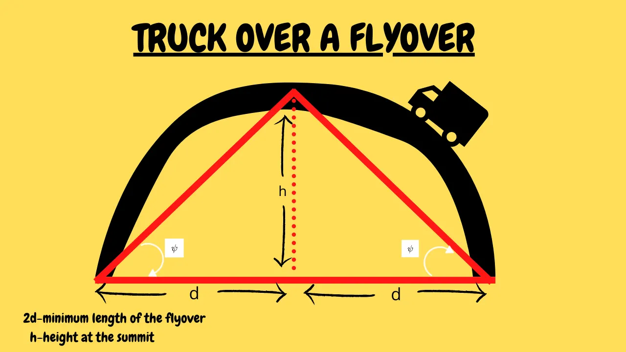
`tan40^0=5.5/d`
`d=(5.5m)/(tan40^0)=6.554m`
minimum length of the flyover`implies``2d=2*6.54m=13.109m`
------------------------------------------------------------------------------------------------------------------------------------------------------------------------------------------------------------------------------------------------------------------------------------------------------------------------------------------------------------------------------------------------------------------------------------------------------------------------------------------------------------------------------------------------------------------------------------------------------------------------------------------------------------------------------------------------------------------------------
OBJECTIVE-3 `implies`Prepare a new drive cycle excel file for the model in the below link and also include a hill-climbing angle to it. Revise the model file “Driver_Glider.slx” and comment on the results `implies` https://in.mathworks.com/matlabcentral/fileexchange/63823-matlab-and-simulink-racing-lounge-vehicle-modeling
THEORY
A driving cycle commonly represents a set of vehicle speed points versus time. It is used to assess fuel consumption and pollutants emissions of a vehicle in a normalized way, so that different vehicles can be compared.
There are two kinds of driving cycles,
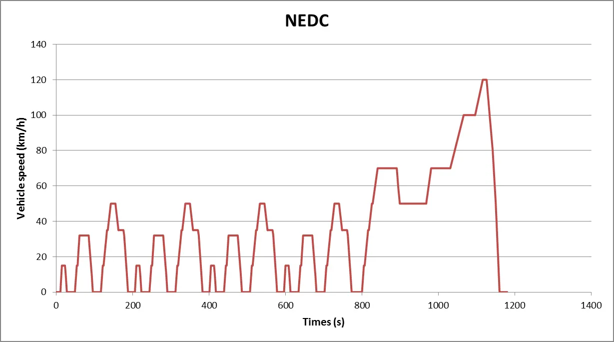
1. Modal cycles `implies`[Eg:-European standard NEDC, or Japanese 10-15 Mode]
2. Transient cycles `implies`[Eg:-FTP-75 or Artemis cycle]
.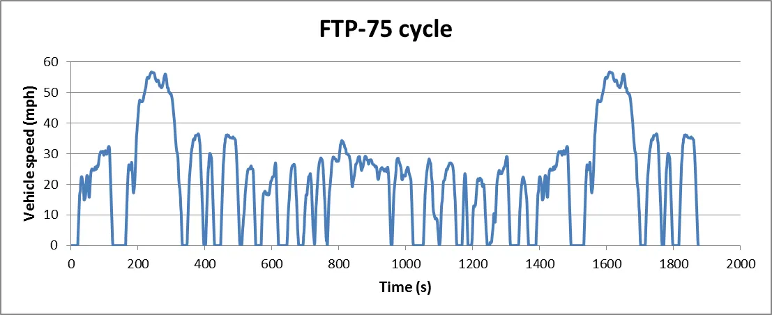
Main difference is that modal cycles are a compilation of straight acceleration and constant speed periods and are not representative of a real driver behavior, whereas transient cycles involve many speed variations, typical of on-road driving conditions.
What is a Traction Force? `implies`the force propelling the vehicle forward, transmitted to the ground through the drive wheels. The force propelling the vehicle forward, the tractive effort, has to accomplish
the following:
1.Rolling Resistance Force `implies``Funderset( rr) ( )=underset( )(mu) underset( rr) ( )mg`→">
2.Aerodynamic Drag Force `implies``Funderset(ad)()=(1/2)(rhoACunderset(D)()V^2)`
3.Hill Climbing Force `Funderset(HC)()=mgsin(psi)`
4.Acceleration due to linear velocity `implies``Funderset(la)()=ma`
5.Acceleration due to angular velocity`implies``Funderset(omegaa)()=G/rT=G/r[IGa/r]=IG^2/r^2a`
6.Total Traction Force `implies``Funderset(TE)()=Funderset(rr)()+Funderset(ad)()+Funderset(hc)()+Funderset(la)()+Funderset(omegaa)()`
PROCEDURE
1. when you click on the above link you will get a compressed file. On extracting the file, you will get some files, which are not the model with connections, instead just an open model or a library where all the required files and blocks for the desired model as shown below:-
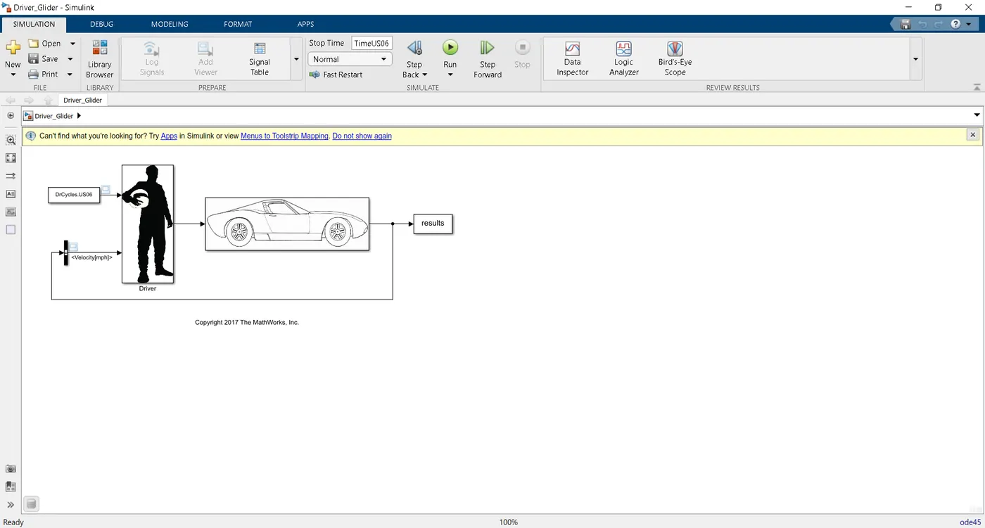
NOTE:-The method to get the model with the required connections as above from it open model or library is clearly defined in the link below:-
https://skill-lync.com/knowledgebase/how-to-open-driver-glider-model-in-simulink
2. You can see there is already an input "DrCycles.US06". This is a drive cycle already defined in the library. But i have mad emy own drive cycle using the excel sheet, as shown below:-

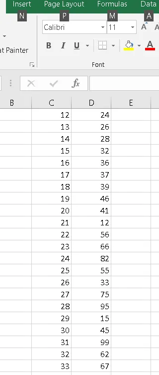
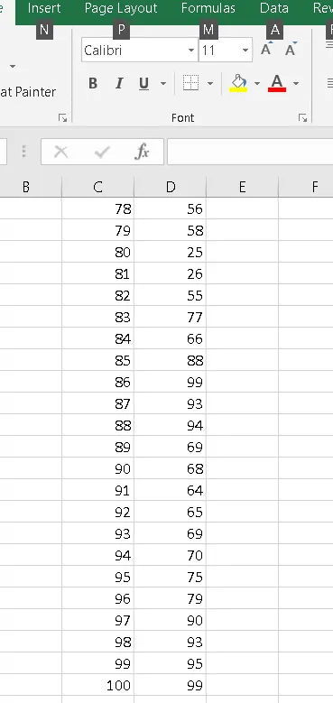
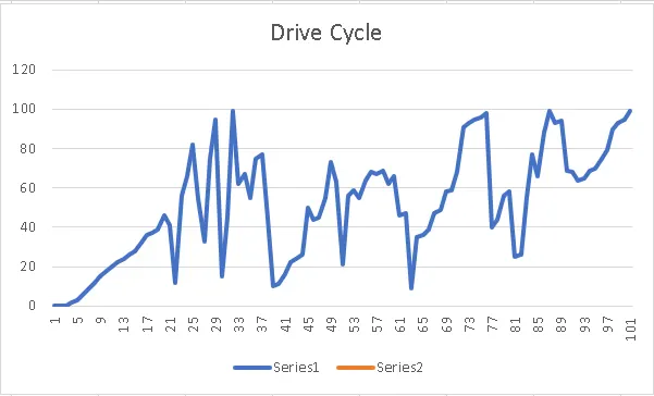
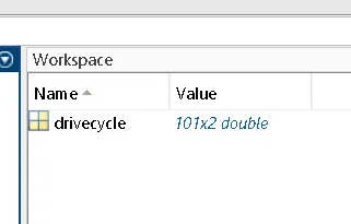
3.I have imported the same excel sheet of drive cycle into matlab as a numeric matrix:-
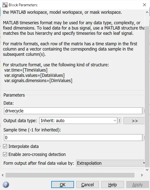
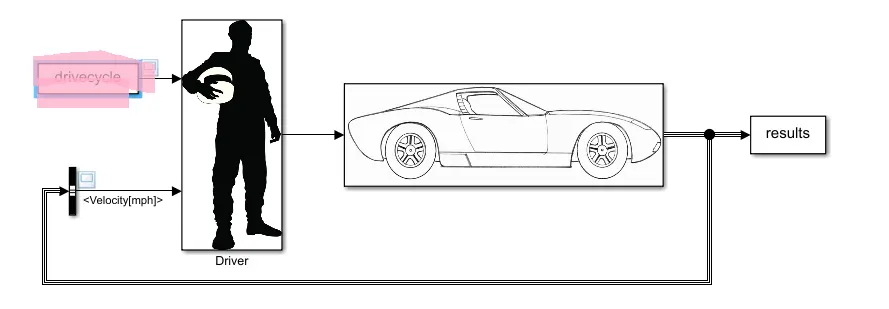
4.Then in the model, this drivecycle is given as input to the "from workspace " block:-
OUTPUT`to`
ANALYSIS
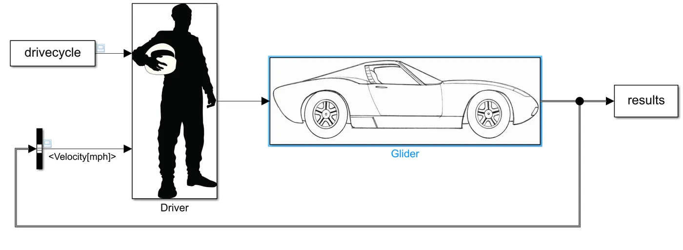
- The input fiven is 2 in numbers. One is the drivecycle and the other is the feedback velocity output as the second output.
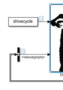
- Then the driver subsystem finds the error by subtracting the two inputs and feeding it into the PID controller block. The PID block is used to find the desired output as close as possible.

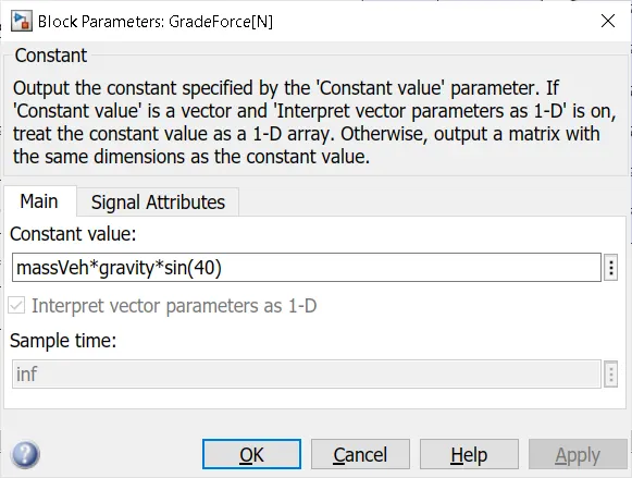
- The glider input is the tractionforce which is used to find the inertia force by the below formula. Also the slope angle is given as `40^0`
`Funderset(i)()=Funderset(tr)()-Funderset(aero)()-Funderset(rr)()-Funderset(gd)()`
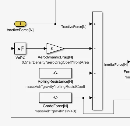
- Then we will find the acceleration, velocity and the position by the formula,
`a=[Funderset(tr)()-Funderset(aero)()-Funderset(gd)()-Funderset(rr)()]/m`

- Then we will find the power and energy from the traction force
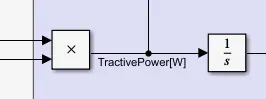
- Now we will use a bus signal that will intake the inputs as tractive power, energy, braking energy, velocity, and the position
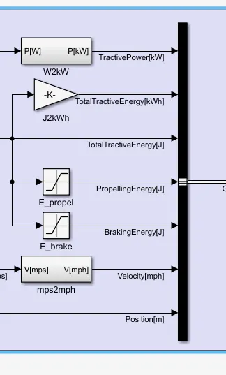
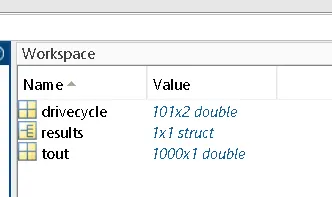
- The final output is stored in the variable as "result", which is stored in the MATLAB workspace
COMPLETE SIMULINK MODEL
OUTCOME OF THE SIMULINK MODEL
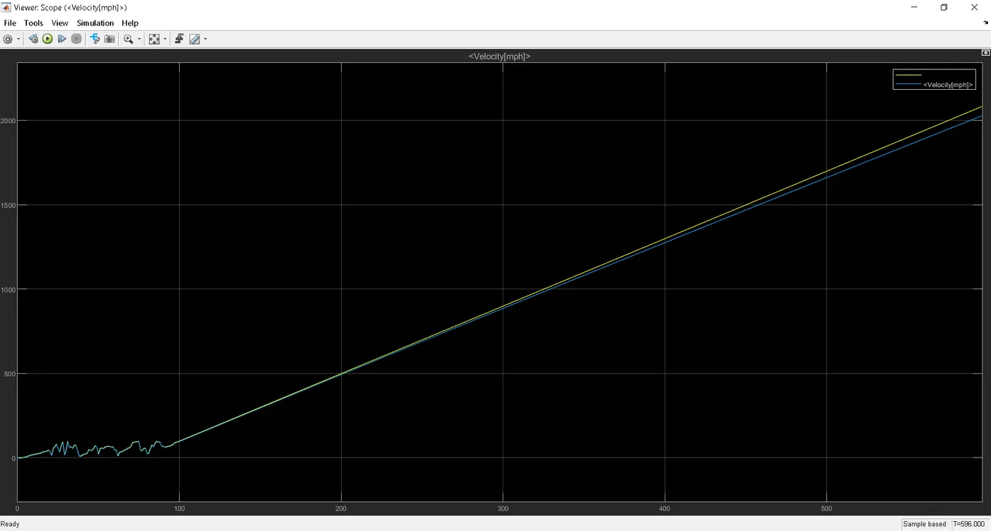
As we have seen the outcome which is similar to the given drive cycle. This makes us understand that the force, power and the energy that is required to the given drive cycle is just adequate and enough for the vehicle to propell without much losss.
REFERENCE
https://skill-lync.com/knowledgebase/how-to-open-driver-glider-model-in-simulink
---------------------------------------------------------------------------------------------------------------------------------------------------------------------------------------------------------------------------------------------------------------------------------------------------------------------------------------------------------------------------------------------------
OBJECTIVE-4 `to` Model the WOT (Wide Open Throttle) response of GM EV1 car. Compare it with the official figures of the performance of a real vehicle. Prepare a table showing variation in acceleration time with a 5% change in vehicle parameters.
PRE-REQUISITES
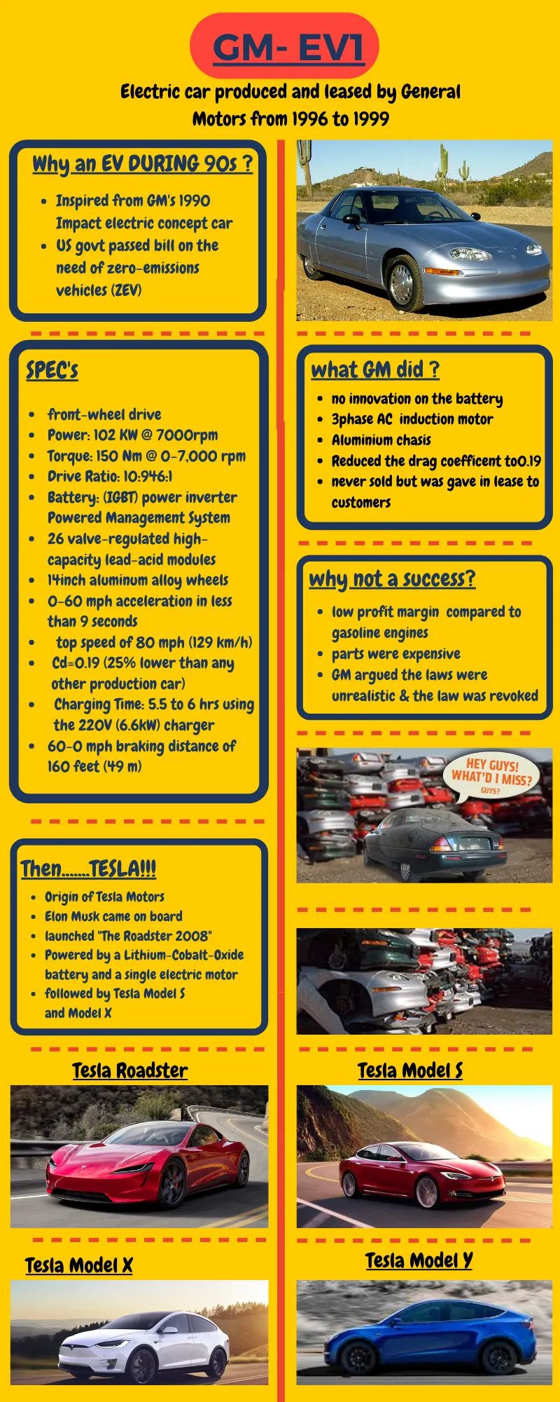
Several years ago, GM has displayed an electric show car named "Impact" in Detroit motor show. In 1997, Impact eventually went into production, but this time called "GM EV1". Very interesting, this innovative car is the first General Motors car sold under the brand "GM", although GM was found as early as 1930's.
EV1 is the first mass production electric car in the world. Electric cars have many technical difficulties, such as the range of running, weight of battery, battery life, performance, charging time and price. Among which, the battery is still the most critical and unsolved problem. The most common lead acid battery is cheap, but it stores little electricity so that the range of running is very limited. Moreover, it takes probably 10 hrs to charge, so you have better to charge your electric car at night. On the contrary, NiMH (Nickel Metal Hybrid) battery is faster to charge and store more energy, but it is so costly that make mass production nonsense. No matter which battery, all of them have short life and they are very heavy ( the battery of EV1 weight as much as 500kg ! ), as a result, performance is considerably deteriorated.
The philosophy of EV1 is sensible : unlike other competitors, EV1 is designed to be an elegant coupe car. If it were an ordinary small sedan, it would be impossible to compete with those more economical and practical petrol cars. A coupe is unnecessary to be practical, nor economical. And its price is less sensitive. Moreover, sophisticated looks, show-car-like interior design and the name "Electric car" help it to grab the heart of some niche buyers.
What GM did?
- In technology, GM has no innovation on the battery. Instead, it optimises the rest of the car to improve performance. For example, its drag coefficient of 0.19 is a world record, breaking the previous record set by Opel Calibra's 0.26 by a large margin.
- It has narrower tyres, no-vent nose and carefully revision in wind tunnel.
- Its electric motor is also very powerful. It is a three phase induction AC motor. The DC supply from the battery should be converted to ac then 3 phase AC before input into the motor, very complicated, but it really allows greater power - 137hp and 149KW maximum
- GM also improved the performance further by reducing weight. Therefore, aluminium space frames chassis is adopted, which is enclosed with a mixture of plastic and glass fiber body panels. Such measures reduce the weight to "only" 1360kg, for a small 2 seats coupe
CASE STUDY-1 `to`Modelling a WOT GM EV1 with real car measurements
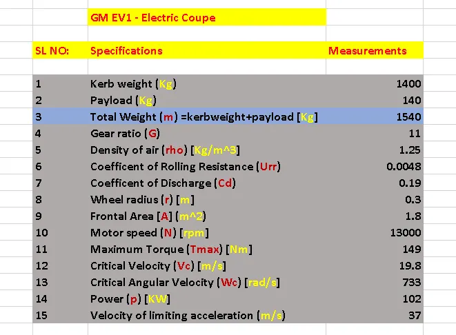
NOTE:- The velocity of limiting acceleration is a company defined value, which can vary as the terrain and road conditions change.
CALCULATION
1. From the traction force equation , we know that:-
`F_(te) = F_(rr) + F_(ad) + F_(la) + F_(omegaa)`
substituting the values of the force terms, we get,
`F_(te) = (mu_{rr}*m*g) + (0.5*rho*A*C_d*v^2) + (m*a) + (I*(G^2/r^2)*(a/ƞ_g))`-----------1
2. Now, the power equation can be defined as:-
`P=tau*omega implies tau*[(v*G)/r]` and
`P=F_(te)*vimpliesF_(te)=P/v=[tau*(v*G)/r]/v=[tau*G]/r`--------------2
Eqn.2 in Eqn.1,
ie. `(T*G)/r = (mu_{rr}*m*g) + (0.5*rho*A*C_d*v^2) + ((m) + I*(G^2/(r^2*ƞ_g)))*((dv)/dt)`------------3
Also the, `I*(G^2/(eta_g*r^2))`term of Eqn3 has to be given the value 20Kg, because of small moment of inertia value for the vehicle. Hence we have considering an approximate value of 20Kg for the term. Then the modified Eqn3 becomes,
`(T_max*G)/r = (mu_{rr}*m*g) + (0.5*rho*A*C_d*v^2) + (m + 20)*(d_v/d_t)`-----------4
3. For most of the motors there are two sets of torque - angular velocity characteristics. From the low speed to a speed called as critical speed, the torque remains constant ad that will be a maximum torque value, then after the critical speed, it starts decreasing exponentially. The graph below is for reference:-
4. So we need two sets of equation:- one for the constant torque region and the other for the constant power region. Both of them can be obtained from Eqn3.
5. The equation constant torque region involves the maximum torque region(ie.`tau_(max)`) So we will subtitute all the given values along with the`tau_(max)=149Nm`Here the the velocity during the maximum torque is obtained from the below defined Eqn5,
ie. `v=2978/tau_(max)=2978/(149Nm)=19.98m/s`
`implies tau=2978/v`----------5
Now Eqn5 can be used in Eqn4 and the remainin values are same as the input values.
NOTE:- The steps 5 and 6 on evaluating will result in differential equation which requires a solver to get the equation. I have used MATLAB as the solver to get the required solution. The MATLAB code is as hown below:-
% MATLAB program for WOT (Wide Open Throttle)on GM(General Motors)-EV1(1st Generation)

clear all              %clears all previous memory in the Workspace
close all              % Close all figures, clean workspace, clean command window
clc                    % clears the command window

m=1540;                % mass of the GM EV1
g=11;                  % gear ratio of GM EV1
rho=1.25;              % density of air
urr=0.0048;            % coefficent of rolling resistance of GM EV1
r=0.3;                 % wheel radius of GM EV1
a=1.8;                 % fronta area of GM EV1
cd=0.19;               % coefficent of discharge of GM EV1


vel=zeros(1,201);      % velocity array

t=linspace(0,50,201);  % time array

dt=0.1;                % time step of 0.1sec for differentiating

for n=1:200                                                                           % for loop for iterative operation to be carried out to find out the velocity values
    if vel(n)<19.98                                                                   % if condition for constant torque region
        tmax=149;                                                                     % maximum torque vaue during the constant torque region
        vel(n+1)=vel(n)+dt*[[[(g*tmax)/r]-[urr*m*g]-[0.5*cd*(vel(n)^2)]]/[m+20]]      % ODE for constant torque region

    elseif vel(n)>=37                                                                 % else-if condition for making the velocity to not go beyond the 37m/s
        vel(n+1)=vel(n);                                                              % making the velocity constant for the above else-if condition

    elseif vel(n)>=19.98                                                              % else-if condition for constant power region
        tmax=2978/vel(n);                                                             % maximum torque vaue during the constant power region
        vel(n+1)=vel(n)+dt*[[[(g*tmax)/r]-[urr*m*g]-[0.5*cd*(vel(n)^2)]]/[m+20]]      % ODE for constant power region
    end                                                                               % whole if-else loop ends
end                                                                                   % for loop ends


vel=vel*3.6;                                        % converting velocity from m/sec to Km/sec
plot(t,vel,'linewidth',1.5,'color','r');            % velocity versus time plot
grid on                                             % grid is made visiblein the plot
xlabel('time(sec)')                                 % x-axis is labelled
ylabel('velocity(km/hr)')                           % y-axis is labelled
title('WOT (Wide Open Throttle) of GM EV1car')      % title is given to the plot
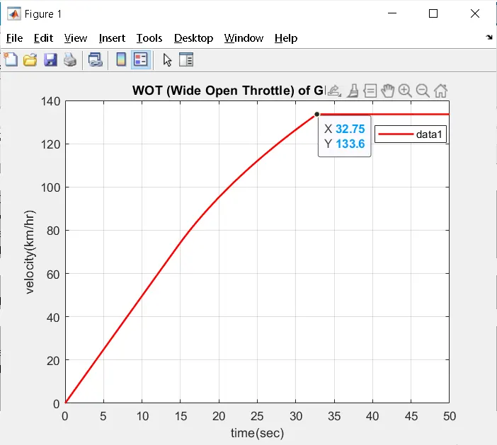
OUTPUT:- You can see the point marked on the graph where the y-axis depicts the velocity as 133.6Km/hr (i.e. 37m/sec)
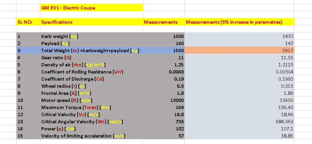
CASE STUDY-2 `to`Modelling a WOT GM EV1 with 5% change (increase) car measurements
CALCULATIONS
Here all the calculations are similar to the case study-1, but only difference comes in step 5 and 6, because of 5% increase in values.
ie. `v=2921/tau_(max)=2921/(156.45Nm)=18.67m/s`
ie. `P=tau*omega implies tau=P/omega=P/((v*G)/r)=156450/((v*11.55)/0.315)=2921/v`
`implies tau=2921/v`
The MATLAB code for the case study-2 is:-
% MATLAB program for WOT (Wide Open Throttle)on GM(General Motors)-EV1(1st
% Generation)with 5% change (Increase) in parametres

clear all              %clears all previous memory in the Workspace
close all              % Close all figures, clean workspace, clean command window
clc                    % clears the command window

m=1617;                % mass of the GM EV1
g=11.55;                  % gear ratio of GM EV1
rho=1.3125;              % density of air
urr=0.00504;            % coefficent of rolling resistance of GM EV1
r=0.315;                 % wheel radius of GM EV1
a=1.89;                 % fronta area of GM EV1
cd=0.1995;               % coefficent of discharge of GM EV1


vel=zeros(1,201);      % velocity array

t=linspace(0,50,201);  % time array

dt=0.1;                % time step of 0.1sec for differentiating

for n=1:200                                                                           % for loop for iterative operation to be carried out to find out the velocity values
    if vel(n)<18.67                                                                   % if condition for constant torque region
        tmax=156.45;                                                                     % maximum torque vaue during the constant torque region
        vel(n+1)=vel(n)+dt*[[[(g*tmax)/r]-[urr*m*g]-[0.5*cd*(vel(n)^2)]]/[m+20]]      % ODE for constant torque region

    elseif vel(n)>=38.85                                                                 % else-if condition for making the velocity to not go beyond the 37m/s
        vel(n+1)=vel(n);                                                              % making the velocity constant for the above else-if condition

    elseif vel(n)>=18.67                                                              % else-if condition for constant power region
        tmax=2921/vel(n);                                                             % maximum torque vaue during the constant power region
        vel(n+1)=vel(n)+dt*[[[(g*tmax)/r]-[urr*m*g]-[0.5*cd*(vel(n)^2)]]/[m+20]]      % ODE for constant power region
    end                                                                               % whole if-else loop ends
end                                                                                   % for loop ends


vel=vel*3.6;                                        % converting velocity from m/sec to Km/sec
plot(t,vel,'linewidth',1.5,'color','r');            % velocity versus time plot
grid on                                             % grid is made visiblein the plot
xlabel('time(sec)')                                 % x-axis is labelled
ylabel('velocity(km/hr)')                           % y-axis is labelled
title('WOT (Wide Open Throttle) of GM EV1car')      % title is given to the plot
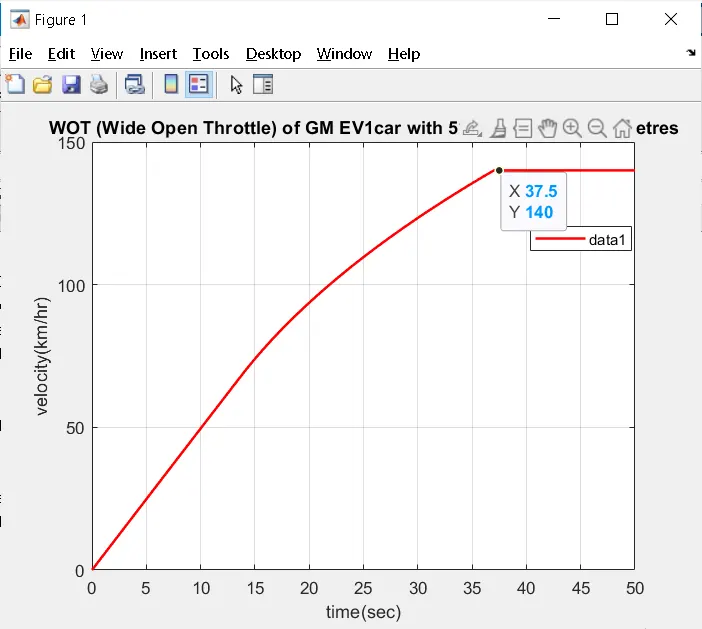
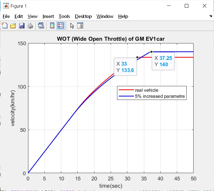
OUTPUT:-You can see the point marked on the graph where the y-axis depicts the velocity as 140Km/hr (i.e. 38.888m/sec)
COMPARISON
Here i have just combined the above 2 case studies and plotted the graph in a single window for better clarity.
CODE:-
% MATLAB program for WOT (Wide Open Throttle)on GM(General Motors)-EV1(1st Generation)

clear all               %clears all previous memory in the Workspace
close all               % Close all figures, clean workspace, clean command window
clc                     % clears the command window

m1=1540;                % mass of the GM EV1
g1=11;                  % gear ratio of GM EV1
rho1=1.25;              % density of air
urr1=0.0048;            % coefficent of rolling resistance of GM EV1
r1=0.3;                 % wheel radius of GM EV1
a1=1.8;                 % fronta area of GM EV1
cd1=0.19;               % coefficent of discharge of GM EV1


vel1=zeros(1,201);      % velocity array

t1=linspace(0,50,201);  % time array

dt1=0.1;                % time step of 0.1sec for differentiating

for i=1:200                                                                                      % for loop for iterative operation to be carried out to find out the velocity values
    if vel1(i)<19.98                                                                             % if condition for constant torque region
        tmax1=149;                                                                               % maximum torque vaue during the constant torque region
        vel1(i+1)=vel1(i)+dt1*[[[(g1*tmax1)/r1]-[urr1*m1*g1]-[0.5*cd1*(vel1(i)^2)]]/[m1+20]]      % ODE for constant torque region

    elseif vel1(i)>=37                                                                           % else-if condition for making the velocity to not go beyond the 37m/s
        vel1(i+1)=vel1(i);                                                                       % making the velocity constant for the above else-if condition

    elseif vel1(i)>=19.98                                                                        % else-if condition for constant power region
        tmax1=2978/vel1(i);                                                                      % maximum torque vaue during the constant power region
        vel1(i+1)=vel1(i)+dt1*[[[(g1*tmax1)/r1]-[urr1*m1*g1]-[0.5*cd1*(vel1(i)^2)]]/[m1+20]]      % ODE for constant power region
    end                                                                                          % whole if-else loop ends
end                                                                                              % for loop ends
vel1=vel1*3.6;                                                                                   % converting velocity from m/sec to Km/sec


% MATLAB program for WOT (Wide Open Throttle)on GM(General Motors)-EV1(1st Generation)with 5% change (Increase) in parametres


m2=1617;                   % mass of the GM EV1
g2=11.55;                  % gear ratio of GM EV1
rho2=1.3125;               % density of air
urr2=0.00504;              % coefficent of rolling resistance of GM EV1
r2=0.315;                  % wheel radius of GM EV1
a2=1.89;                   % fronta area of GM EV1
cd2=0.1995;                % coefficent of discharge of GM EV1


vel2=zeros(1,201);         % velocity array


dt2=0.1;                   % time step of 0.1sec for differentiating

for i=1:200                                                                                       % for loop for iterative operation to be carried out to find out the velocity values
    if vel2(i)<18.67                                                                              % if condition for constant torque region
        tmax2=156.45;                                                                             % maximum torque vaue during the constant torque region
        vel2(i+1)=vel2(i)+dt2*[[[(g2*tmax2)/r2]-[urr2*m2*g2]-[0.5*cd2*(vel2(i)^2)]]/[m2+20]]      % ODE for constant torque region

    elseif vel2(i)>=38.85                                                                         % else-if condition for making the velocity to not go beyond the 37m/s
        vel2(i+1)=vel2(i);                                                                        % making the velocity constant for the above else-if condition

    elseif vel2(i)>=18.67                                                                         % else-if condition for constant power region
        tmax2=2921/vel2(i);                                                                       % maximum torque vaue during the constant power region
        vel2(i+1)=vel2(i)+dt2*[[[(g2*tmax2)/r2]-[urr2*m2*g2]-[0.5*cd2*(vel2(i)^2)]]/[m2+20]]      % ODE for constant power region
    end                                                                                           % whole if-else loop ends
end                                                                                               % for loop ends


vel2=vel2*3.6;                                        % converting velocity from m/sec to Km/sec
plot(t1,vel1,'linewidth',1.5,'color','r');            % velocity versus time plot
hold on
plot(t1,vel2,'linewidth',1.5,'color','b');            % velocity versus time plot
grid on                                               % grid is made visiblein the plot
xlabel('time(sec)')                                   % x-axis is labelled
ylabel('velocity(km/hr)')                             % y-axis is labelled
title('WOT (Wide Open Throttle) of GM EV1car')        % title is given to the plot
legend('real vehicle','5% increased parametre')       % legend is created
INFERENCE:-We see that the critical velocity has increased on increasing the parametres by 5%. Without increase it was 133.33Km/s and after increasing by 5%, it has become140Km/s.
IMPORTANT FILES
- https://drive.google.com/file/d/1sfXRcZj2zQpIOwtDCnVenZ_yZLZLJnvQ/view?usp=sharing
- https://drive.google.com/file/d/1IVURN4w-TGk-gPxiAQMz5nq80I97ElHh/view?usp=sharing
- https://drive.google.com/file/d/1KvZYBRD1SKw15LctdHPmnoEpoCILw4zF/view?usp=sharing
- Whole files in one compressed file:-https://drive.google.com/drive/folders/1980jJZ14MheUV-6B62bd5r08-1LwkiIj?usp=sharing
REFERENCE
https://www.torque.com.sg/reviews/general-motors-ev1-was-an-advanced-electric-car/
http://www.autozine.org/Archive/GM/old/EV1.html
https://www.motortrend.com/news/general-motors-ev1/
http://www.evchargernews.com/CD-A/gm_ev1_web_site/specs/specs_specs.htm