MATLAB solver for the steady and unsteady 2D heat conduction problem
AIM `to`
Solve the 2D heat conduction equation by using the point iterative techniques for both STEADY and UNSTEADY equations. The Boundary conditions for the problem are as follows;
Top Boundary = 600 K
Bottom Boundary = 900 K
Left Boundary = 400 K
Right Boundary = 800 K
You will implement the following methods for solving implicit equations.
1. Jacobi
2. Gauss-seidel
3. Successive over-relaxation
Your absolute error criteria is 1e-4
PRE-REQUISITES `to`
3D Heat Conduction Equation 'to``(partial T)/(partial t) - alpha*((partial^2 T)/(partial x^2) + (partial^2 T)/(partial y^2) + (partial^2 T)/(partial z^2) ) - (alpha*dotq_G)/K= 0`
where `alphato`thermal diffusivity.
2D Heat Conduction Equation `to` `(partial T)/(partial t) - alpha*((partial^2 T)/(partial x^2) + (partial^2 T)/(partial y^2) ) = 0`
Before getting into the above two equations , we need to know certain terms. The above equations can be generalized in terms of TRANSPORT Equations. The transport equation describes how a scalar quantity is transported in a space. Usually, it is applied to the transport of a scalar field (e.g. chemical concentration, material properties or temperature) inside an incompressible flow. From the mathematical point of view, the transport equation is also called the convection-diffusion equation, which is a first-order PDE (partial differential equation). The convection-diffusion equation is the basis for the most common transportation models.
Generally, Transport equation `implies` Continuity Equation (i.e. mass as the scalar field) `implies` conservation of mass
what is Continuity Equation? `implies` the rate of change for a scalar quantity in any differential control volume is given by the flow and diffusion of the scalar into and out of the system, along with any generation or consumption inside the control volume. Or, the variation of concentration of a certain quantity in the volume is given by the balance of this quantity flow across the boundary and the amount of quantity produced or removed in the volume. Mathematically,
`frac{partial c}{partial t}+nabla cdot j=S`,
where `cto`scalar field, `jto`flux of `c`, `Sto` source/sink term inside the control volume.
- `(partial c)/(partial t) to` time-dependent variation of the scalar field inside the C.V.
- `nabla cdot j to`net balance of the quantity which enters and exits the C.V.
- `Sto` amount of the scalar quantity “created” or “destroyed” inside the C.V.
Flux `j` can be divided into two terms: the convective and the diffusive terms.
i.e. j = Convective terms + Diffusive term
= (moves across the boundaries of the C.V, hence, proportional to velocity) + (transportation of the scalar quantity according to its gradient)
`j`= `(c*u)` + `(Dnablac)`,
where `Dto` diffusivity
Also, `S` = (Pure source term) + (Reaction Term)
= (the creation/destruction rate of the field inside the volume) + ( the creation/destruction of the transported quantity as a reaction to this quantity itself, theredore, is a function of transport field `c`)
Note `to` Reaction source term is is quite uncommon for engineering applications and is often neglected.
Therefore, `frac{partial c}{partial t}+ nablacdot (uc)+nablacdot(Dnabla c)=S`
So, here the transport field is TEMPERATURE `(T)`
`frac{partial T}{partial t}+ nablacdot (uT)+nablacdot(alpha*nabla T)=S`
where `alpha` is the thermal diffusivity
Now, as per the requirements, we are not taking any quantities outside the C.V and will stick with the 2D. Therefor, the CONVECTIVE term in the temperature flux (i.e. `nablacdot(uT)`) is neglected, as well as the Source term. Hence, we are left with the equation as shown below `implies`
For UNSTEADY Case `to`
`frac{partial T}{partial t}+nablacdot(alpha*nabla T)=0 implies frac{partial T}{partial t}+(alpha*nabla^2 T)=0``implies` `(partial T)/(partial t) - alpha*((partial^2 T)/(partial x^2) + (partial^2 T)/(partial y^2) ) = 0`
For STEADY Case `to`
`((partial^2 T)/(partial x^2) + (partial^2 T)/(partial y^2) ) = 0`
METHODS OF FINDING THE SOLUTIONS `to`
The above equations have second order partial derivatives. And since we are using the computers to solve the equations. For that we need to descretize these partial derivatives which will eventually, form a system of linear algebraic equations. There are two families of solution techniques for linear algebraic equations:
- direct methods and
- Indirect or Iterative methods
Simple examples of direct methods are Cramer’s rule matrix inversion and Gaussian elimination.
Iterative methods are based on the repeated application of a relatively simple algorithm leading to eventual convergence after a large number of repetitions. Well-known examples are the Jacobi and Gauss–Seidel and Reaxation Methods. The total number of operations, typically of
the order of N per iteration cycle, cannot be predicted in advance. Stronger still, it is not possible to guarantee convergence unless the system of equations satisfies fairly exacting criteria. The main advantage of iterative solution methods is that only non-zero coefficients of the equations need to be stored in core memory.
These methods are differentiated based on the usage of values of interation. To understand this, consider a 5-noded imaginary space as shown below. The computational domain is assigned with the boundary conditions as shown. Here, we need to solve the governing equation (i.e. 2D Heat equation) at each nodes. Hence, this is an iterative technique.
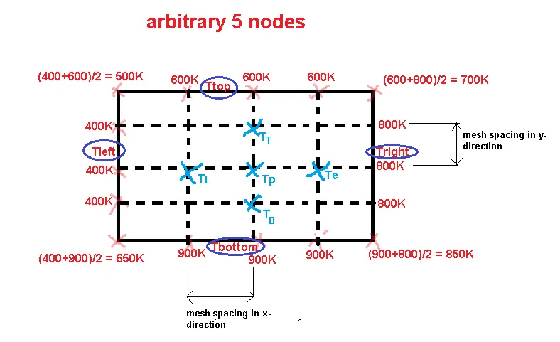
In most computing machines, the calculations are performed sequentially, so we will start the sequence of calculations by using the initial guess as `T_1^(0) = T_2^(0) = T_3^(0) =0`
Jacobi Method `to` In the Jacobi method the right hand side is evaluated using the results of the previous iteration or from the initial guess. For example, the temperature at the Kth time step will be based on values of (K-1)th iterations.
i.e. `T^(K)=I*T^(K-1) +c`,
where `Ito` Iteration Matrix and `cto` constant vector
Gauss-Siedal Method `to` the Gauss–Seidel method continues to use the most up-to-date values on the right hand side that are available. So
i.e. `T^(K)=T_1^(K) + T_2^(K-1)+c`,
Here, the temperature at node 1 for the time step (K), `T_1^(K)` is used instead of `T_1^(K-1)`
Relaxation Methods `to` The convergence rate of the Jacobi and Gauss–Seidel methods depends on the properties of the iteration matrix. It has been found that these can be a improved by the introduction of a so-called relaxation parameter `omega`.
If `omega=1implies` Jacobi Method
`0<omega<1 implies` Under-relaxation Mathod
`omega>1 implies` Over-relaxation Method
Also, we have another classification on how to solve the differential equations `to` Explicit and Implicit Schemes. When a direct computation of the dependent variables can be made in terms of known quantities, the computation is said to be explicit. When the dependent variables are defined by coupled sets of equations, and either a matrix or iterative technique is needed to obtain the solution, the numerical method is said to be implicit.
DESCRETIZING OF THE 2D HEAT CONDUCTION EQUATION (UNSTEADY) `to`
NOTE `to` Here I have used Unsteady equation, as it will include every partial derivatives, so, Forward Differencing scheme `to` `(partial T)/(partial t )` and
Central Differencing Scheme `to` `(partial^2 T)/(partial x^2)` & `(partial^2 T)/(partial y^2)`
`therefore` `(T_(i,j)^(n+1) _T_(i,j)^(n))/(triangle t) + alpha * ((T_(i+1,j) - 2T_(i,j) - T_(i-1,j))/(triangle x^2) + (T_(i,j+1) - 2T_(i,j) - T_(i,j-1))/(triangle y^2)) = 0`.......................Unsteady case
The below two schemes are for unsteady case`implies`
EXPLICIT SCHEME `implies`
`implies(T_(i,j)^(n+1) - T_(i,j)^(n))/(triangle t) + alpha * (((T_(i+1,j) - 2T_(i,j) - T_(i-1,j))/(triangle x^2))^n + ((T_(i,j+1) - 2T_(i,j) - T_(i,j-1))/(triangle y^2))^n) = 0`
`implies T_(i,j)^(n+1) = T_(i,j)^(n) + (alpha *triangle t) *(((T_(i+1,j) - 2T_(i,j) - T_(i-1,j))/(triangle x^2) )^(n)+ ((T_(i,j+1) - 2T_(i,j) - T_(i,j-1))/(triangle y^2))^(n))`
`implies` `T_(i,j)^(n+1) = T_(i,j)^(n) + [(alpha *triangle t)/(triangle x^2) *(T_(i+1,j) - 2T_(i,j) - T_(i-1,j))^(n)] + [(alpha *triangle t)/(triangle y^2) * (T_(i,j+1) - 2T_(i,j) - T_(i,j-1))^(n)] `
Let CFL in x and y direction be `implies`
`implies``CFL_X = (alpha*triangle t) / (triangle x^2)`
`implies``CFL_y = (alpha*triangle t) / (triangle y^2)`
`implies``T_w=T_(i,j+1)`
`implies``T_E = T_(i,j+1)`
`implies``T_T=T_(i-1,j)`
`implies``T_S = T_(i+1,j)`
`therefore T_P^(n+1) = T_P^(n) + [CFL_x *(T_S - 2T_P + T_T)^(n)] + [CFL_y * (T_W - 2T_P + T_E)^(n)]`
`implies``T_P^(n+1) = (1 - 2CFL_x - 2CFL_y)*T_P^(n) + [CFL_x*(T_S + T_T)^n ]+ [CFL_y*(T_E + T_W)^n]`
IMPLICIT SCHEME `implies`
`implies (T_(i,j)^(n+1) _T_(i,j)^(n))/(triangle t) + alpha * (((T_(i+1,j) - 2T_(i,j) - T_(i-1,j))/(triangle x^2))^(n+1) + (T_(i,j+1) - 2T_(i,j) - T_(i,j-1))/(triangle y^2))^(n+1)) = 0`
On rearranging `to`
`implies T_(i,j)^(n+1) = T_(i,j)^(n) + (alpha *triangle t) *(((T_(i+1,j) - 2T_(i,j) - T_(i-1,j))/(triangle x^2) )^(n+1)+ ((T_(i,j+1) - 2T_(i,j) - T_(i,j-1))/(triangle y^2))^(n+1))`
`implies` `T_(i,j)^(n+1) = T_(i,j)^(n) + [(alpha *triangle t)/(triangle x^2) *(T_(i+1,j) - 2T_(i,j) - T_(i-1,j))^(n+1)] + [(alpha *triangle t)/(triangle y^2) * (T_(i,j+1) - 2T_(i,j) - T_(i,j-1))^(n+1)] `
Let CFL in x and y direction be `implies`
`CFL_X = (alpha*triangle t) / (triangle x^2)`
`CFL_y = (alpha*triangle t) / (triangle y^2)`
`T_w=T_(i,j+1)`
`T_E = T_(i,j+1)`
`T_T=T_(i-1,j)`
`T_S = T_(i+1,j)`
`therefore T_P^(n+1) = T_P^(n) + [CFL_x *(T_S - 2T_P + T_T)^(n+1)] + [CFL_y * (T_W - 2T_P + T_E)^(n+1)]`
`implies` `T_P(n+1) = T_P^(n) - [2*CFL_x*T_P^(n+1)] - [2*CFL_y*T_P^(n+1)] + [CFL_x(T_S +T_T)^(n+1)] + [CFL_y(T_W +T_E)^(n+1)]`
`implies` `(1+ 2*CFL_x + 2*CFL_y) * T_P(n+1) = T_P^n + [CFL_x(T_S +T_T)^(n+1)] + [CFL_y(T_W +T_E)^(n+1)]`
`implies` `T_P(n+1) =(1/(1+ 2*CFL_x + 2*CFL_y))*( T_P^n + [CFL_x(T_S +T_T)^(n+1)] + [CFL_y(T_W +T_E)^(n+1)])`
DESCRETIZING OF THE 2D HEAT CONDUCTION EQUATION (STEADY) `to`
`implies``((T_(i+1,j) - 2T_(i,j) - T_(i-1,j))/(triangle x^2) + (T_(i,j+1) - 2T_(i,j) - T_(i,j-1))/(triangle y^2)) = 0`.................................Steady case
`implies``T_P = (1/(K)) * ((T_W+T_E)/(triangle x^2) + (T_S+T_T)/(triangle y^2) )`
where `K = [((triangle x^2) * (triangle x^2)) / ((triangle x^2) + (triangle x^2))]`
ALGORITHM `to`
There will be a main program which will ask for user-defined inputs. In total there are 7 cases. Therefore, I have used 7 functions, individually for each cases. The cases are as follows `implies`
- Steady Jacobi Method
- Steady Gauss-Siedal Method
- Steady Successove Over-Relaxation Method (SOR)
- Unsteady Explicit Method
- Unsteady Implicit Jacobi Method
- Unsteady Implicit Gauss-Siedal Method
- Unsteady Implicit SOR Method
Algorithm for MAIN program code `to`
% 2D Heat Conduction Equation Solver for Both Steady and Unsteady state, using % % JACOBI, GAUSS-SIEDAL & SOR Iterative Methods


% previous plots and figures are closed
% preivious variables from the workspace are deleted
% previous results are cleared from the command window


% user is asked to enter the following =>
    % Type of method
    %number of nodes in x and y directions


% the Boundary Conditions are defined
    % here the temperature specifications at each sides are the BC's

% Initialising the problem
    % the node points other than the side nodes, that is the nodes at the
    % bulk are initialised by 300K


% if-else loop is defined
    % the loop is for executing each methods in an organised way as per the
    % user's requirement. Each method is defined inside a function
    % Therefore, they are called from the corresponding if-else conditions
Algorithm for each Steady state methods `to`
% corresponding STEADY method heading

% function handle is defined

% inputs are defined such as =>
     %domain lenth
     % mesh in x and y direction
     % mesh spacing in x and y direction
     % the constant k which comes in each methods equation
     % iterations


% inputs for error calculations => this are defined because the solution obtained should be of high accuracy. So there should be some standard/limit upto which the iterations should run, so that the converged results are of high accuracy


% loop to run the program till convergence. Here the code runs till the error
  value goes below the threshold value.
       {
            { %space loop => Since we have to compute for 2D case, we need 2
                             `for` loops to define the rows and coloumns. Both
                             the for loop starts from the index number `2`,
                             becoz, the `1` is already covered in BC's. The for
                             loop ends till the index number `1 less than the
                             number of nodes in x and y direction`.
              Statements inside for loop => equations corresponding to each
                                            Methods
            }

          %error value is calulated and updated
          %the teperature values are updated
       }


% the contours are plotted
Algorithm for UNSTEADY case `to`
% corresponding UNSTEADY method heading

% function handle is defined

% inputs are defined such as =>
     %domain lenth
     % mesh in x and y direction
     % mesh spacing in x and y direction
     % the constant k which comes in each methods equation
     % iterations


% inputs for error calculations => this are defined because the solution obtained
  should be of high accuracy. So there should be some standard/limit upto which the
  iterations should run, so that the converged results are of high accuracy


% time loop is defind for unsteady case
   {
     % loop to run the program till convergence. Here the code runs till the error
        value goes below the threshold value.
            {
                   { %space loop => Since we have to compute for 2D case, we need 2
                             `for` loops to define the rows and coloumns. Both
                             the for loop starts from the index number `2`,
                             becoz, the `1` is already covered in BC's. The for
                             loop ends till the index number `1 less than the
                             number of nodes in x and y direction`.
                     Statements inside for loop => equations corresponding to each
                                            Methods
                   }

                  %error value is calulated and updated
                  %the teperature values are updated
             }

    }

% the contours are plotted
PROGRAM
Main Program
% 2D Heat Conduction Equation Solver for Both Steady and Unsteady state, using JACOBI, GAUSS-SIEDAL & SOR
% Iterative Methods

%%
close all
clear all
clc

%%
%Asking the user to enter the input values
Question ='What type of heat conduction equation is preferred?- 1)STEADY or 2)UNSTEADY';
user_input_value = input(Question);
number_of_nodes_in_x_direction = input("enter the number of nodes needed in X direction- ");
number_of_nodes_in_y_direction = input("enter the number of nodes needed in Y direction- ");


%%
%Defining the Temperature Domain & Boundary Conditions the problem
    %Top Boundary
    T_initial(1,1)=500;                                                       %average of top and left boundaries
    T_initial(1,(2:(number_of_nodes_in_y_direction-1)))=600;                  %top side nodes from coloumns 2 to 4
    T_initial(1,number_of_nodes_in_y_direction)=700;                          %average of top and right boundaries

    %Left Boundary
    T_initial((2:(number_of_nodes_in_x_direction-1)),1)=400;                    %left side nodes from rows 2 to 4
    T_initial(number_of_nodes_in_x_direction,1)=650;                            %average of right and bottom boundaries

    %Bottom Boundary
    T_initial(number_of_nodes_in_x_direction,(2:(number_of_nodes_in_y_direction-1)))=900;                %bottom side nodes from coloumns 2 to 4
    T_initial(number_of_nodes_in_x_direction,number_of_nodes_in_y_direction)=850;                        %average of bottom and right boundaries

    %Right Boundary
    T_initial((2:(number_of_nodes_in_x_direction-1)),number_of_nodes_in_y_direction)=800;                %right side nodes from rows 2 to 4

%%
%Initialising the problem
    T_initial((2:(number_of_nodes_in_x_direction-1)),(2:(number_of_nodes_in_y_direction-1)))=300;
    T_old = T_initial;
              %the 2d matrix created for solving the 2d heat eqn. is
              %initialsied. This initialization is for those cells which
              %are not in boundary conditions.

%%
%Choice of Iterative Solver for STEADY state heat conduction equation
%The if-else conditions is for deciding whether the user require the solution for
%STEADY or UNSTEADY equation, and from there nested if-else loops are
%defined to decide the coice of iterative solver (ie.JACOBI or GAUSS-SIEDEL or SOR)

    if user_input_value == 1                                        %for STEADY state heat conduction equation

            text = input("Since the chosen preference is STEADY state heat conduction equation,... press enter,");
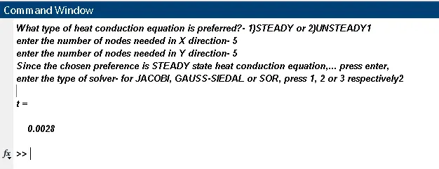
            solver_set_1=input("enter the type of solver- for JACOBI, GAUSS-SIEDAL or SOR, press 1, 2 or 3 respectively");

                    if solver_set_1 == 1                            %Nested if-else conditions for choice of iterative solver for Steady case.
                        T=steady_jacobi(T_old,number_of_nodes_in_x_direction,number_of_nodes_in_y_direction,T_initial);

                    elseif solver_set_1 == 2
                        T=steady_gauss_siedal(T_old,number_of_nodes_in_x_direction,number_of_nodes_in_y_direction,T_initial);

                    elseif solver_set_1 == 3
                        T=steady_SOR(T_old,number_of_nodes_in_x_direction,number_of_nodes_in_y_direction,T_initial);
                        return;

                    end
    else                                                              %For UNSTEADY / TRANSIENT state heat conduction equation

        fprintf('The chosen preference is UNSTEADY / TRANSIENT state heat conduction equation')
        schemes=input("enter the choice for- 1)EXPLICIT schemes or 2)IMPLICIT schemes")
                    if schemes == 1           %Nested if-else conditions to decide whether Explicit or Implicit Scheme
                                              %This if condition is for Explicit Scheme.
                       %solver_set_2=input("enter the type of solver for EXPLICIT scheme- for JACOBI, GAUSS-SIEDAL or SOR, press 1, 2 or 3 respectively");
                         T=unsteady_explicit(T_old,number_of_nodes_in_x_direction,number_of_nodes_in_y_direction,T_initial);

                    else                                                %This if condition is for Implicit Scheme.

                         solver_set_3=input("enter the type of solver for IMPLICIT scheme- for JACOBI, GAUSS-SIEDAL or SOR, press 1, 2 or 3 respectively");

                                if solver_set_3 == 1  %Nested if-else condition for deciding the type of Iterative Solver.
                                    T=unsteady_implicit_jacobi(T_old, number_of_nodes_in_x_direction, number_of_nodes_in_y_direction, T_initial);

                                elseif solver_set_3 == 2
                                    T=unsteady_implicit_gauss_siedal(T_old,number_of_nodes_in_x_direction,number_of_nodes_in_y_direction,T_initial);

                                elseif solver_set_3 == 3
                                    T=unsteady_implicit_SOR(T_old,number_of_nodes_in_x_direction,number_of_nodes_in_y_direction,T_initial);
                                    return;

                                end
                    end
    end
Function for STEADY CASES `to`
STEADY Jacobi Method `to`
`implies``T_P = (1/(K)) * ((T_W^(old)+T_E^(old))/(triangle x^2) + (T_S^(old)+T_T^(old))/(triangle y^2) )`, where `K = [((triangle x^2) * (triangle x^2)) / ((triangle x^2) + (triangle x^2))]`
%function for STEADY JACOBI Iterative Method to solve the 2D heat conduction
%equation

function [T_new] = steady_jacobi(T_old,number_of_nodes_in_x_direction,number_of_nodes_in_y_direction,T_new)

%Inputs required
    domain_length = 1;
    mesh_in_x_direction = linspace(0,domain_length,number_of_nodes_in_x_direction);
    mesh_in_y_direction = linspace(0,domain_length,number_of_nodes_in_y_direction);
    mesh_spacing_in_x_direction = mesh_in_x_direction(2)- mesh_in_x_direction(1);
    mesh_spacing_in_y_direction = mesh_in_y_direction(2)- mesh_in_y_direction(1);
    k=2*(((mesh_spacing_in_x_direction^2)+(mesh_spacing_in_y_direction^2))/((mesh_spacing_in_x_direction^2)*(mesh_spacing_in_y_direction^2)));
    iterations = 0;

%%
%Error Calculations
error_magnitude = 1;                     %initialising the error magnitude to enter into the while loop
error_required = 1e-04;                  %threshold error value

%%
%Calculations for JACOBI method
tic
   %convergence loop
    while error_magnitude > error_required
       %space loop
        for i=2:(number_of_nodes_in_x_direction-1)      %Row Number
            for j=2:(number_of_nodes_in_y_direction-1)  %coloumn loop
                iterations = iterations + 1;             %number of iterations
                term_1(i,j)= ((T_old(i,j+1)+ T_old(i,j-1))/(mesh_spacing_in_x_direction^2));
                term_2(i,j) = ((T_old(i+1,j)+ T_old(i-1,j))/(mesh_spacing_in_y_direction^2));
                T_new(i,j)= (term_1(i,j)+term_2(i,j))/k;      %temperature value at the new point
            end
        end
            error_magnitude = max(max(abs(T_old-T_new)));  %error or residual calculation for convergence criteria
            T_old = T_new;                                 %the old temperature values are upedated

    end

    t=toc
    [X,Y]=meshgrid(mesh_in_x_direction,mesh_in_y_direction);
    [C,h]=contourf(mesh_in_x_direction,mesh_in_y_direction,T_new,25);   %contours are potted
    set(gca, 'YDir','reverse')            %for reversing the y-direction, as the
                                          %temperature values were not in sync with the BC's
    grid on
    clabel(C,h)
    colormap(jet)
    colorbar
    xlabel('x-axis')
    ylabel('y-axis')
    zlabel('Temperature')
    title(sprintf('steady state- (Jacobi method)- No: of Iterations=%d',iterations))
end
STEADY Guass-Siedal Method `to`
`implies``T_P = (1/(K)) * ((T_W^(New)+T_E^(old))/(triangle x^2) + (T_S^(old)+T_T^(New))/(triangle y^2) )`, where `K = [((triangle x^2) * (triangle x^2)) / ((triangle x^2) + (triangle x^2))]`
%function for STEADY GAUSS-SIEDAL Iterative Method to solve the 2D heat conduction
%equation


function [T_new] = steady_gauss_siedal(T_old,number_of_nodes_in_x_direction,number_of_nodes_in_y_direction,T_new)

%Inputs required
    domain_length = 1;
    mesh_in_x_direction = linspace(0,domain_length,number_of_nodes_in_x_direction);
    mesh_in_y_direction = linspace(0,domain_length,number_of_nodes_in_y_direction);
    mesh_spacing_in_x_direction = mesh_in_x_direction(2)- mesh_in_x_direction(1);
    mesh_spacing_in_y_direction = mesh_in_y_direction(2)- mesh_in_y_direction(1);
    k=2*(((mesh_spacing_in_x_direction^2)+(mesh_spacing_in_y_direction^2))/((mesh_spacing_in_x_direction^2)*(mesh_spacing_in_y_direction^2)));
    iterations = 0;

%%
%Error Calculations
error_magnitude = 1;              %initialising the error magnitude to enter into the while loop
error_required = 1e-04;           %threshold error value

%%
%Calculations for GAUSS-SIEDAL method
tic
    %Convergence Loop
    while error_magnitude > error_required
       %Space Loop
        for i=2:(number_of_nodes_in_x_direction-1)  %Row Numbers
            for j=2:(number_of_nodes_in_y_direction-1)   %Coloumn Numbers
                iterations = iterations + 1;                %number of iterations
                term_1(i,j) = ((T_old(i,j+1)+ T_new(i,j-1))/(mesh_spacing_in_x_direction^2));
                term_2(i,j) = ((T_old(i+1,j)+ T_new(i-1,j))/(mesh_spacing_in_y_direction^2));
                T_new(i,j)= (term_1(i,j)+term_2(i,j))/k;    %temperature value at the new point
            end
        end
            error_magnitude = max(max(abs(T_old-T_new)));   %error or residual calculation for convergence criteria
            T_old = T_new;                                  %the old temperature values are upedated
    end
        display(T_new)
    t=toc
    [X,Y]=meshgrid(mesh_in_x_direction,mesh_in_y_direction);
    [C,h]=contourf(mesh_in_x_direction,mesh_in_y_direction,T_new,25);   %contours are potted
    set(gca, 'YDir','reverse')                          %for reversing the y-direction, as the
                                                        %temperature values were not in sync with the BC's
    grid on
    clabel(C,h)                                         %labeling the contour
    colormap(jet)
    colorbar
    xlabel('x-axis')
    ylabel('y-axis')
    zlabel('Temperature')
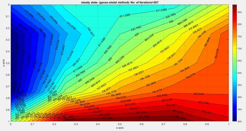
    title(sprintf('steady state- (gauss-siedal method)- No: of Iterations=%d',iterations))
end
STEADY SOR Method `to`
`implies``T_P^(n+1) = (1-omega)T_P^(old) + omega*T_(GS)`,
where `omegato` relaxation factor and `T_(GS) = (1/(K)) * ((T_W^(New)+T_E^(old))/(triangle x^2) + (T_S^(old)+T_T^(New))/(triangle y^2) )`
`K = [((triangle x^2) * (triangle x^2)) / ((triangle x^2) + (triangle x^2))]`
%function for STEADY SOR Iterative Method to solve the 2D heat conduction
%equation

function [T_new] = steady_SOR(T_old,number_of_nodes_in_x_direction,number_of_nodes_in_y_direction,T_new)

%Inputs required
    domain_length = 1;
    mesh_in_x_direction = linspace(0,domain_length,number_of_nodes_in_x_direction);
    mesh_in_y_direction = linspace(0,domain_length,number_of_nodes_in_y_direction);
    mesh_spacing_in_x_direction = mesh_in_x_direction(2)- mesh_in_x_direction(1);
    mesh_spacing_in_y_direction = mesh_in_y_direction(2)- mesh_in_y_direction(1);
    k=2*(((mesh_spacing_in_x_direction^2)+(mesh_spacing_in_y_direction^2))/((mesh_spacing_in_x_direction^2)*(mesh_spacing_in_y_direction^2)));
    iterations = 0;

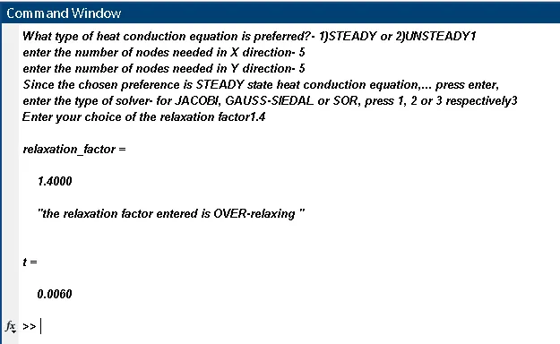
    relaxation_factor = input("Enter your choice of the relaxation factor")

    if relaxation_factor > 1
        display("the relaxation factor entered is OVER-relaxing ")
    elseif relaxation_factor < 1
        display("the relaxation factor entered is UNDER-relaxing ")
    else
        display("the default relaxation factor is 0.7")
        relaxation_factor=0.7;
    end

%%
%Error Calculations
error_magnitude = 1;              %initialising the error magnitude to enter into the while loop
error_required = 1e-04;           %threshold error value

%%
%Calculations for JACOBI method
tic
    while error_magnitude > error_required
        for i=2:(number_of_nodes_in_x_direction-1)
            for j=2:(number_of_nodes_in_y_direction-1)
                iterations = iterations + 1;                 %temperature value at the new point
                term_1(i,j) = ((T_old(i,j+1)+ T_new(i,j-1))/(mesh_spacing_in_x_direction^2));
                term_2(i,j) = ((T_old(i+1,j)+ T_new(i-1,j))/(mesh_spacing_in_y_direction^2));
                T_gauss_siedal(i,j) = (term_1(i,j)+term_2(i,j))/k;
                T_new(i,j)= (((1-relaxation_factor)*T_old(i,j)) + (relaxation_factor*T_gauss_siedal(i,j)));
                                                 %temperature value at the new point
            end
        end
            error_magnitude = max(max(abs(T_old-T_new)));        %error or residual calculation for convergence criteria
            T_old = T_new;                                       %the old temperature values are upedated
    end

    t=toc
    [X,Y]=meshgrid(mesh_in_x_direction,mesh_in_y_direction);
    [C,h]=contourf(mesh_in_x_direction,mesh_in_y_direction,T_new,25);   %contours are potted
    set(gca, 'YDir','reverse')                 %for reversing the y-direction, as the
                                               %temperature values were not in sync with the BC's
    grid on
    clabel(C,h)                                %labeling the contour plot
    colormap(jet)
    colorbar
    xlabel('x-axis')
    ylabel('y-axis')
    zlabel('Temperature')
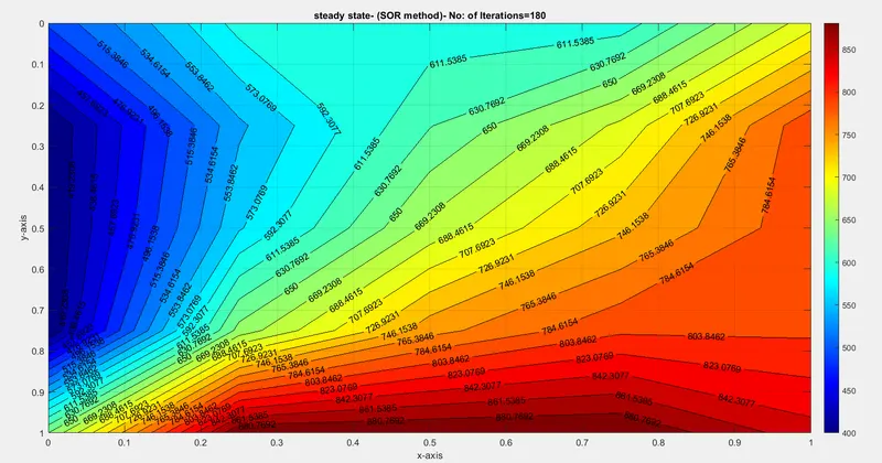
    title(sprintf('steady state- (SOR method)- No: of Iterations=%d',iterations))
end
UNSTEADY Explicit Method `to` Here there so need to find solutons using Iterative methods, since the RHS is already known and only LHS is to calculated. Hence every method is applicable.
`implies``T_P^(n+1) = (1 - 2CFL_x - 2CFL_y)*T_P^(old) + [CFL_x*(T_S + T_T)^(old) ]+ [CFL_y*(T_E + T_W)^(old)]`,
`implies``CFL_X = (alpha*triangle t) / (triangle x^2)`
`implies``CFL_y = (alpha*triangle t) / (triangle y^2)`
%function for UNSTEADY EXPLICIT Method to solve the 2D heat conduction
%equation


function [T_new] = unsteady_explicit(T_old,number_of_nodes_in_x_direction,number_of_nodes_in_y_direction,T_new)

%Inputs required
    domain_length = 1;
    mesh_in_x_direction = linspace(0,domain_length,number_of_nodes_in_x_direction);
    mesh_in_y_direction = linspace(0,domain_length,number_of_nodes_in_y_direction);
    mesh_spacing_in_x_direction = mesh_in_x_direction(2)- mesh_in_x_direction(1);
    mesh_spacing_in_y_direction = mesh_in_y_direction(2)- mesh_in_y_direction(1);
    iterations = 0;
    alpha = 0.0001;
    dt=0.01;

%%
%CFL calculation
 CFL_x = (alpha*dt)/(mesh_spacing_in_x_direction^2);
 CFL_y = (alpha*dt)/(mesh_spacing_in_y_direction^2);
 CFL = CFL_x + CFL_y;

%%
%Calculations for unsteady explicit method
tic
%time loop
 for nt=1:1400
       %space loop
        for i=2:(number_of_nodes_in_x_direction-1)           %row loop
            for j=2:(number_of_nodes_in_y_direction-1)       %coloumn loop
                display(i)
                display(j)

                term_1(i,j)= (T_old(i,j+1))- (2*T_old(i,j))+ (T_old(i,j-1));
                term_2(i,j)= (T_old(i+1,j))- (2*T_old(i,j))+ (T_old(i-1,j));
                T_new(i,j)= T_old(i,j)+ (CFL_x*term_1(i,j)) + (CFL_y*term_2(i,j));
                                               %temperature value at the new point
            end
        end
            T_old = T_new;                     %the old temperature values are upedated
            iterations = iterations + 1;       %number of iterations
 end

    t=toc
    [X,Y]=meshgrid(mesh_in_x_direction,mesh_in_y_direction);
    [C,h]=contourf(mesh_in_x_direction,mesh_in_y_direction,T_new,25);   %contours are potted
    set(gca, 'YDir','reverse')                  %for reversing the y-direction, as the
                                                %temperature values were not in sync with the BC's
    grid on
    clabel(C,h)                                 %labeling the contour
    colormap(jet)
    colorbar
    xlabel('x-axis')
    ylabel('y-axis')
    zlabel('Temperature')
    title(sprintf('Unsteady state- No: of Iterations=%d',iterations))
end
UNSTEADY Implicit Jacoby `to`
`implies` `T_P(n+1) =(1/(1+ 2*CFL_x + 2*CFL_y))*( T_P^(prev) + [CFL_x(T_S +T_T)^(old)] + [CFL_y(T_W +T_E)^(old)])`
`implies``CFL_X = (alpha*triangle t) / (triangle x^2)`
`implies``CFL_y = (alpha*triangle t) / (triangle y^2)`
%function for UNSTEADY IMPLICIT JACOBI Iterative Method to solve the 2D heat conduction
%equation


function [T_new] = unsteady_implicit_jacobi(T_old, number_of_nodes_in_x_direction, number_of_nodes_in_y_direction, T_new)

%Inputs required
    domain_length = 1;
    mesh_in_x_direction = linspace(0,domain_length,number_of_nodes_in_x_direction);
    mesh_in_y_direction = linspace(0,domain_length,number_of_nodes_in_y_direction);
    mesh_spacing_in_x_direction = mesh_in_x_direction(2)- mesh_in_x_direction(1);
    mesh_spacing_in_y_direction = mesh_in_y_direction(2)- mesh_in_y_direction(1);
    iterations = 0;
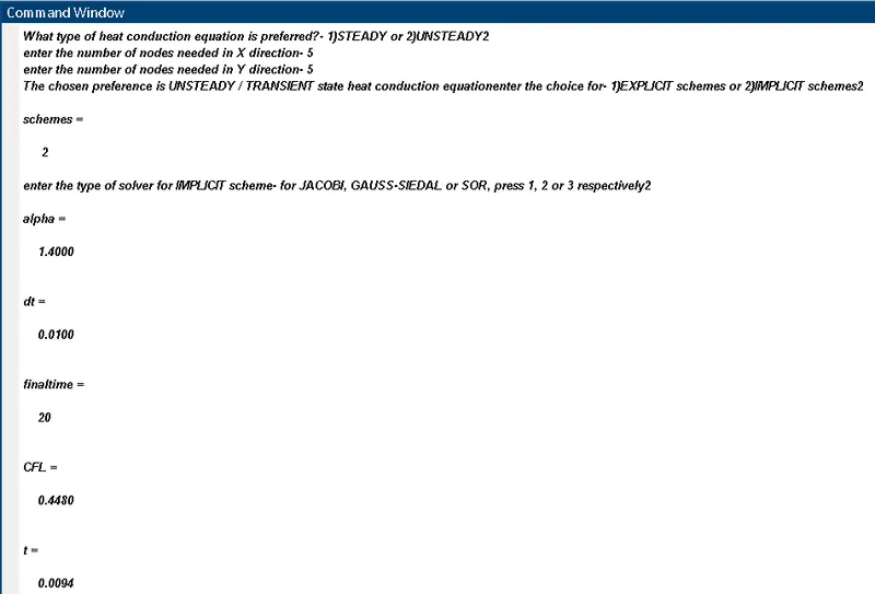
    alpha = 1.4                         %thermal diffusivity
    dt=1e-02                            %end time limit
    finaltime = 20                      %number of time steps
    time_vector = 0:dt:finaltime;
    T_prev = T_old;
%%
%Error Calculations
    error_magnitude = 1;              %initialising the error magnitude to enter into the while loop
    error_required = 1e-04;           %threshold error value

%%
%CFL calculation
     CFL_x = (alpha*dt)/(mesh_spacing_in_x_direction^2);
     CFL_y = (alpha*dt)/(mesh_spacing_in_y_direction^2);
     CFL = CFL_x + CFL_y

%%
%Calculations for UNSTEADY IMPLICIT JACOBI method
%const = 1/(1 + (2*CFL_x) + (2*CFL_y));
    tic
       %Time Loop
       for nt=1:length(time_vector)
          error_magnitude = 1;
           %convergence loop
           while error_magnitude > error_required
                %space loop
                for i=2:(number_of_nodes_in_x_direction-1)  %Row Number
                    for j=2:(number_of_nodes_in_y_direction-1) %Coloum Number

                          term1 = (1+(2*CFL_x)+(2*CFL_y))^(-1);
                          term2= CFL_x*term1;
                          term3= CFL_y*term1;
                          H=(T_old(i-1,j)+T_old(i+1,j));
                          v=(T_old(i,j-1)+T_old(i,j+1));
                          T_new(i,j)= (T_prev(i,j)*term1)+term2*H+term3*v;

                    end
                end
                error_magnitude = max(max(abs(T_old-T_new)));  %error or residual calculation for convergence criteria
                T_old = T_new;                                 %the old temperature values are upedated
                iterations = iterations + 1;                   %number of iterations

           end
           T_prev = T_new;
       end

    t=toc
    [X,Y]=meshgrid(mesh_in_x_direction,mesh_in_y_direction);
    [C,h]=contourf(mesh_in_x_direction,mesh_in_y_direction,T_new,25);   %contours are potted
    set(gca, 'YDir','reverse')            %for reversing the y-direction, as the
                                          %temperature values were not in sync with the BC's
    grid on
    clabel(C,h)
    colormap(jet)
    colorbar
    xlabel('x-axis')
    ylabel('y-axis')
    zlabel('Temperature')
    title(sprintf('Unsteady state- (Jacobi method)- No: of Iterations=%d',iterations))
end
UNSTEADY Implicit Gauss-Siedal`to`
`implies` `T_P(n+1) =(1/(1+ 2*CFL_x + 2*CFL_y))*( T_P^(prev) + [CFL_x(T_S^(old) +T_T^(New)] + [CFL_y(T_W^(New) +T_E^(old)])`
`implies``CFL_X = (alpha*triangle t) / (triangle x^2)`
`implies``CFL_y = (alpha*triangle t) / (triangle y^2)`
%function for UNSTEADY IMPLICIT GAUSS-SIEDAL Iterative Method to solve the 2D heat conduction
%equation


function [T_new] = unsteady_implicit_gauss_siedal(T_old, number_of_nodes_in_x_direction, number_of_nodes_in_y_direction, T_new)

%Inputs required
    domain_length = 1;
    mesh_in_x_direction = linspace(0,domain_length,number_of_nodes_in_x_direction);
    mesh_in_y_direction = linspace(0,domain_length,number_of_nodes_in_y_direction);
    mesh_spacing_in_x_direction = mesh_in_x_direction(2)- mesh_in_x_direction(1);
    mesh_spacing_in_y_direction = mesh_in_y_direction(2)- mesh_in_y_direction(1);
    iterations = 0;
    alpha = 1.4                     %thermal diffusivity
    dt=1e-02                        %end time limit
    finaltime = 20                  %number of time steps
    time_vector = 0:dt:finaltime;
    T_prev = T_old;
%%
%Error Calculations
    error_magnitude = 1;              %initialising the error magnitude to enter into the while loop
    error_required = 1e-04;           %threshold error value

%%
%CFL calculation
     CFL_x = (alpha*dt)/(mesh_spacing_in_x_direction^2);
     CFL_y = (alpha*dt)/(mesh_spacing_in_y_direction^2);
     CFL = CFL_x + CFL_y

%%
%Calculations for UNSTEADY IMPLICIT GAUSS-SIEDAL method

    tic
          %Time Loop
           for nt=1:length(time_vector)
              error_magnitude = 1;
              %convergence loop
               while error_magnitude > error_required
                   %space loop
                    for i=2:(number_of_nodes_in_x_direction-1)  %Row Number
                        for j=2:(number_of_nodes_in_y_direction-1) %Coloum Number

                              term1 = (1+(2*CFL_x)+(2*CFL_y))^-1;
                              term2= CFL_x*term1;
                              term3= CFL_y*term1;
                              H=(T_new(i-1,j)+T_old(i+1,j));
                              v=(T_new(i,j-1)+T_old(i,j+1));
                              T_new(i,j)= T_prev(i,j)*term1+term2*H+term3*v;

                        end
                    end
                    error_magnitude = max(max(abs(T_old-T_new)));  %error or residual calculation for convergence criteria
                    T_old = T_new;                                 %the old temperature values are upedated
                    iterations = iterations + 1;                   %number of iterations

               end
               T_prev = T_new;
           end

    t=toc
    [X,Y]=meshgrid(mesh_in_x_direction,mesh_in_y_direction);
    [C,h]=contourf(mesh_in_x_direction,mesh_in_y_direction,T_new,25);   %contours are potted
    set(gca, 'YDir','reverse')            %for reversing the y-direction, as the
                                          %temperature values were not in sync with the BC's
    grid on
    clabel(C,h)
    colormap(jet)
    colorbar
    xlabel('x-axis')
    ylabel('y-axis')
    zlabel('Temperature')
    title(sprintf('Unsteady state- (Gauss-Siedal method)- No: of Iterations=%d',iterations))
end
UNSTEADY Implicit SOR`to`
`implies``T_P^(n+1) = (1-omega)T_P^(old) + omega*T_(GS)`,
where `omegato` relaxation factor and `T_(GS) =(1/(1+ 2*CFL_x + 2*CFL_y))*( T_P^(prev) + [CFL_x(T_S^(old) +T_T^(New)] + [CFL_y(T_W^(New) +T_E^(old)])`
`implies``CFL_X = (alpha*triangle t) / (triangle x^2)`
`implies``CFL_y = (alpha*triangle t) / (triangle y^2)`
%function for UNSTEADY IMPLICIT SOR Iterative Method to solve the 2D heat conduction
%equation


function [T_new] = unsteady_implicit_SOR(T_old, number_of_nodes_in_x_direction, number_of_nodes_in_y_direction, T_new)

%Inputs required
    domain_length = 1;
    mesh_in_x_direction = linspace(0,domain_length,number_of_nodes_in_x_direction);
    mesh_in_y_direction = linspace(0,domain_length,number_of_nodes_in_y_direction);
    mesh_spacing_in_x_direction = mesh_in_x_direction(2)- mesh_in_x_direction(1);
    mesh_spacing_in_y_direction = mesh_in_y_direction(2)- mesh_in_y_direction(1);
    iterations = 0;
    alpha = 1.4                      %thermal diffusivity
    dt=1e-02                         %end time limit
    finaltime = 20                   %number of time steps
    time_vector = 0:dt:finaltime;
    T_prev = T_new;

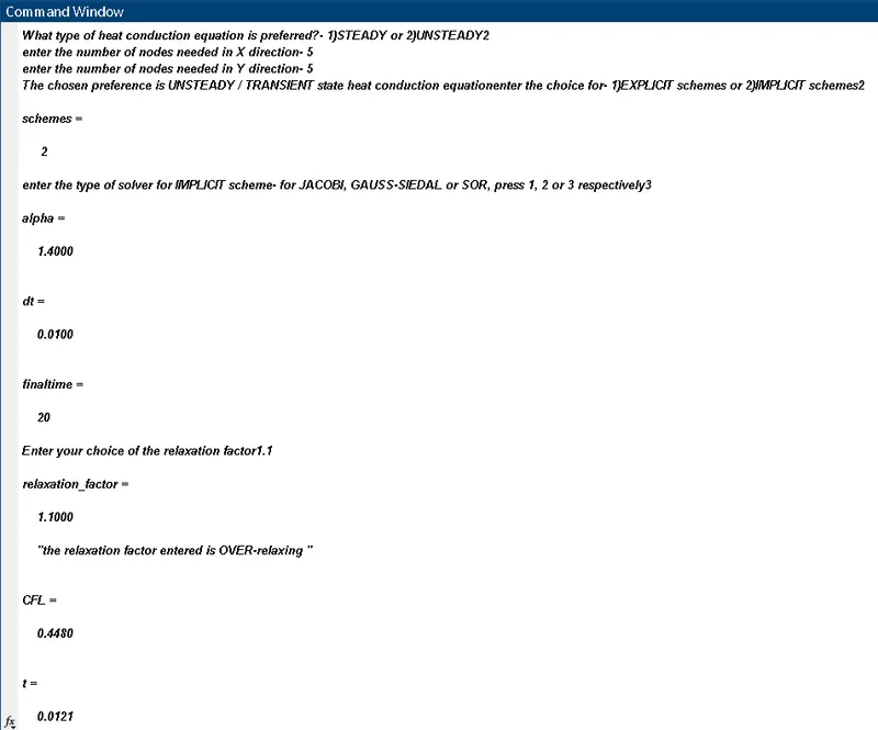
    relaxation_factor = input("Enter your choice of the relaxation factor")

    if relaxation_factor > 1
        display("the relaxation factor entered is OVER-relaxing ")
    elseif relaxation_factor < 1
        display("the relaxation factor entered is UNDER-relaxing ")
    else
        display("the default relaxation factor is 0.7")
        relaxation_factor=0.7;
    end
%%
%Error Calculations
    error_magnitude = 1;              %initialising the error magnitude to enter into the while loop
    error_required = 1e-04;           %threshold error value

%%
%CFL calculation
     CFL_x = (alpha*dt)/(mesh_spacing_in_x_direction^2);
     CFL_y = (alpha*dt)/(mesh_spacing_in_y_direction^2);
     CFL = CFL_x + CFL_y

%%
%Calculations for UNSTEADY IMPLICIT SOR method
    tic
       %Time Loop
       for nt=1:length(time_vector)
           %convergence loop
          error_magnitude = 1;
           while error_magnitude > error_required
                %space loop
                for i=2:(number_of_nodes_in_x_direction-1)  %Row Number
                    for j=2:(number_of_nodes_in_y_direction-1) %Coloum Number

                          term1 = (1+(2*CFL_x)+(2*CFL_y))^-1;
                          term2= CFL_x*term1;
                          term3= CFL_y*term1;
                          H=(T_new(i-1,j)+T_old(i+1,j));
                          v=(T_new(i,j-1)+T_old(i,j+1));
                          T_gauss_siedal(i,j)= (T_prev(i,j)*term1) + (term2*H) + (term3*v);
                          T_new(i,j)= (((1-relaxation_factor)*T_old(i,j))+ (relaxation_factor*T_gauss_siedal(i,j)));
                    end
                end
                error_magnitude = max(max(abs(T_old-T_new)));  %error or residual calculation for convergence criteria
                T_old = T_new;                                 %the old temperature values are upedated
                iterations = iterations + 1;                   %number of iterations

           end
           T_prev = T_new;
       end

    t=toc
    [X,Y]=meshgrid(mesh_in_x_direction,mesh_in_y_direction);
    [C,h]=contourf(mesh_in_x_direction,mesh_in_y_direction,T_new,25);   %contours are potted
    set(gca, 'YDir','reverse')            %for reversing the y-direction, as the
                                          %temperature values were not in sync with the BC's
    grid on
    clabel(C,h)
    colormap(jet)
    colorbar
    xlabel('x-axis')
    ylabel('y-axis')
    zlabel('Temperature')
    title(sprintf('Unsteady state- (SOR method)- No: of Iterations=%d',iterations))
end
RESULTS `to`
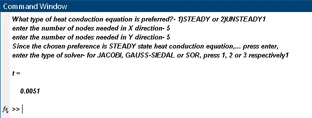
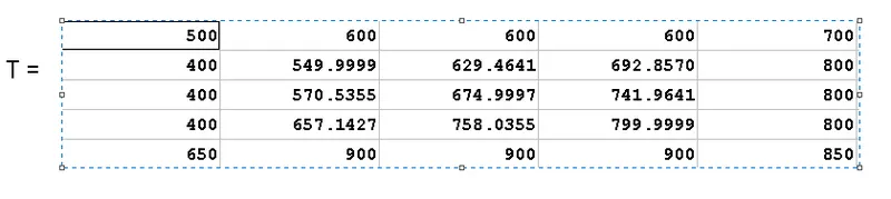
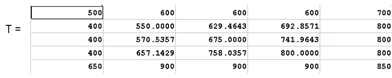
Temperature matrix of (5x5) `to` Each cell can be visualised as a node.

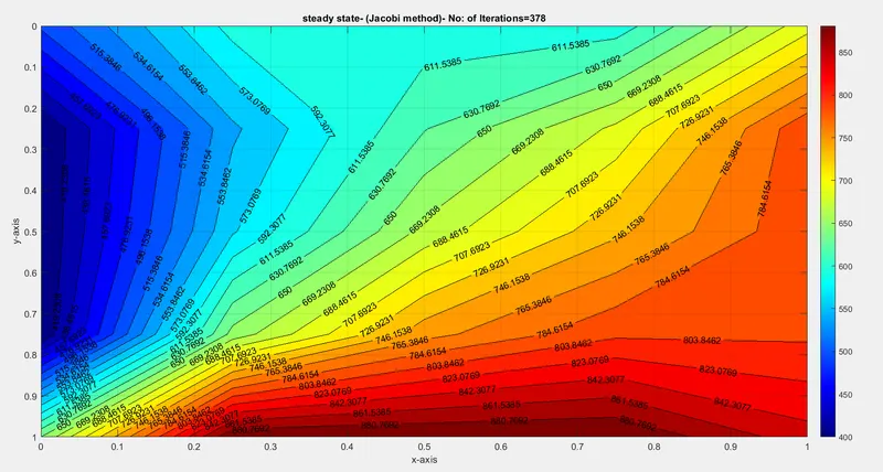
Steady JACOBI method `to`
Steady GAUSS-SIEDAL method `to`

Steady SOR method `to`

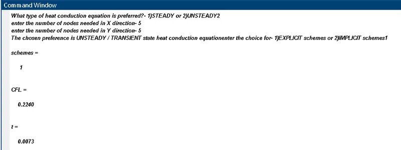
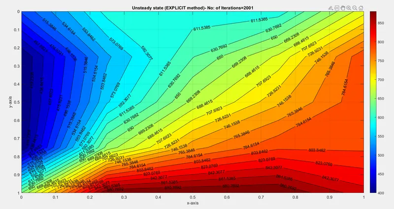
Unsteady EXPLICIT method `to`

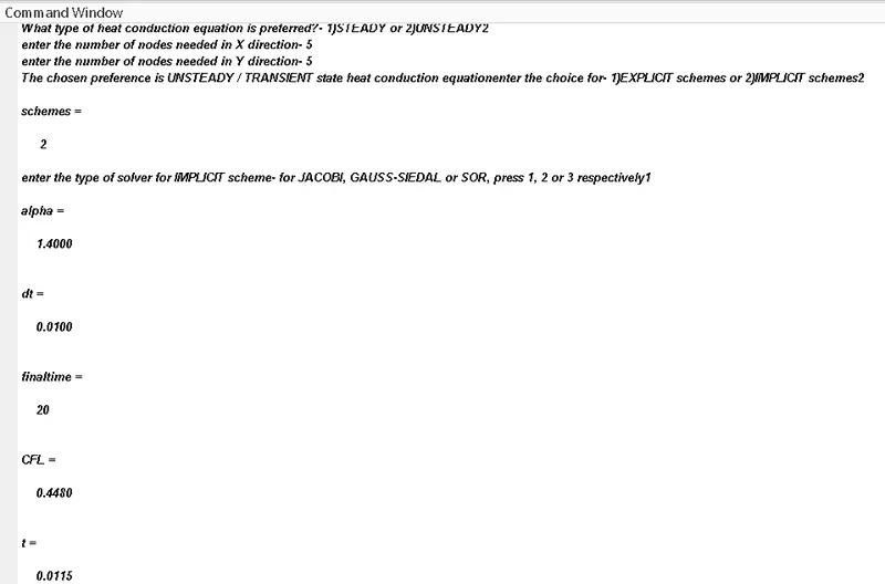
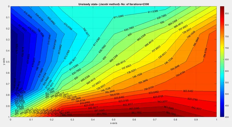
Unsteady IMPLICIT JACOBI method `to`
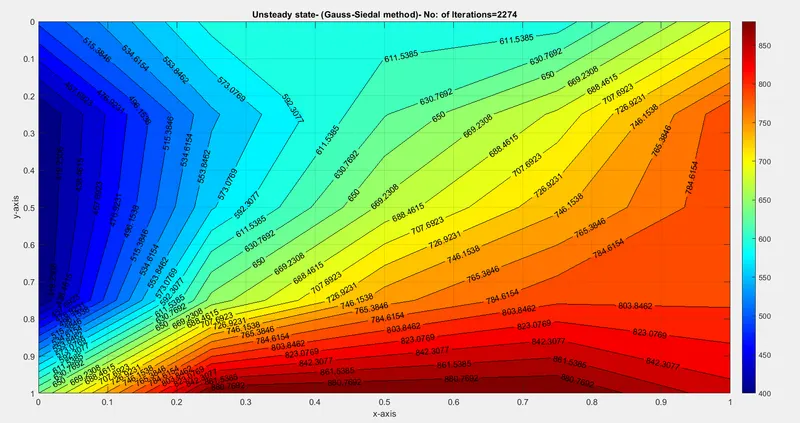
Unsteady IMPLICIT GAUSS-SIEDAL method `to`

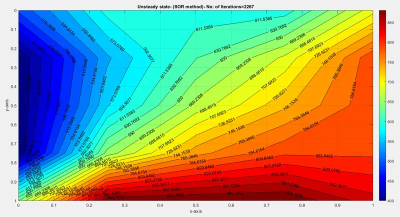
Unsteady IMPLICIT SOR method `to`

CONCLUSION `to`
- The plots shown abpve for every case is not actually smooth and curvy. It has sharp edges. It is because the numbr of nodes = 5. If it is increased, the plot will be more curvy.
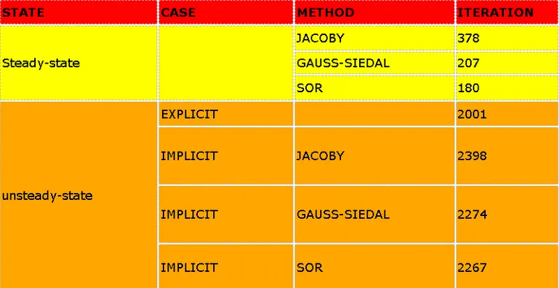
- The steady state SOR & unsteady Implicit SOR has least iterations when compared with other 2 methods, because of relaxation factor.
- The solution temperature matrix (i.e. T ) for each method is same .
REFERENCE `to`
https://www.simscale.com/docs/simwiki/numerics-background/what-is-the-transport-equation/