Parametric Steady State Simulation on Gate valve Using Ansys Fluent.

Aim:

The major objective was to set up a Steady State simulation on the Gate valve and perform a parametric study by setting the opening from 10 % to 80% using Ansys fluent.

The main objective is further subdivided into sub-objective:-

• Estimating the mass flow rates at the outlet for each design point.
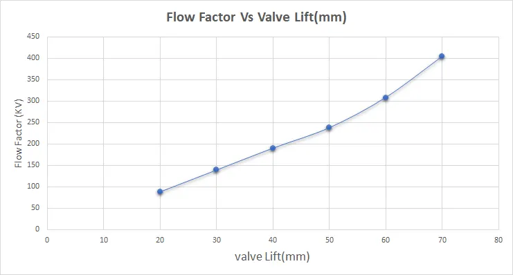
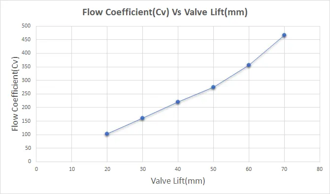
• Determining the flow coefficient and flow factor for each opening and plot the graph.
• Analyzing results of the mass flow rate and flow coefficient.

Introduction:

A gate valve, also known as a sluice valve, is a valve that opens by lifting a barrier (gate) out of the path of the Fluid. Gate valves require very little space along the pipe axis and hardly restrict the flow of fluid when the gate is fully opened. The gate faces can be parallel but are most commonly wedge-shaped (in order to be able to apply pressure on the sealing surface).

Gate valves are used to shut off the flow of liquids rather than for flow regulation. When fully open, the typical gate valve has no obstruction in the flow path, resulting in very low Flow resistance. The size of the open flow path generally varies in a nonlinear manner as the gate is moved. This means that the flow rate does not change evenly with stem travel. Depending on the construction, a partially open gate can vibrate from the fluid flow.

Gate valves are mostly used with larger pipe diameters (from 2" to the largest pipelines) since they are less complex to construct than other types of valves in large sizes.

1. Geometry Creation:

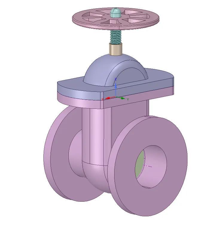
The Gate Valve Geometry was designed using a separate cad package using Solidworks. Then the geometry was imported to Ansys design modular for future control volume creation as it defines the fluid flow domain. The fluid flow domain was prepared using the volume preparation option in fluent. The gate valve was set to paramteric mode.

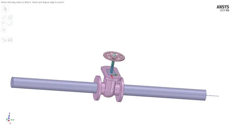
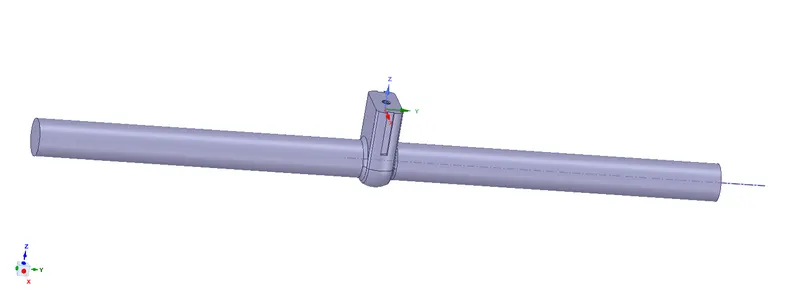
The left and right side of the Control volume domain was extruded to 800mm assuming it as a long pipe connected with gate valve.

2. Boundary Creation and Meshing

After the control volumes are perfectly created the boundary tags were created in order to assign the different boundary conditions ie. velocity, temperature(if needed), or some other physics. For this geometry, 2 different boundary tags or names were created that were used earlier to assign the boundary condition. The 2 names are Inlet and outlet. The remaining walls was set to walls by deafult.

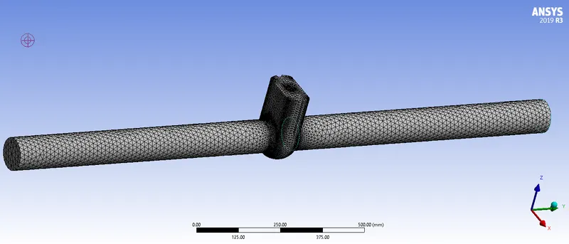
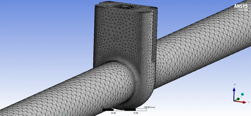
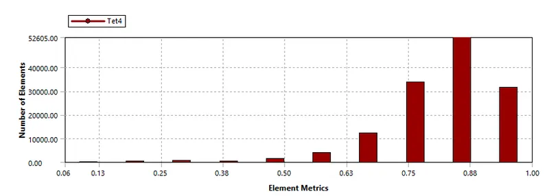
Tet Shape mesh was generated as the flow was aligned and especially the flow was turbulent.

The Mesh was generated using 20mm Base mesh Size.

Number of Elements	136470
Number of Nodes	28819

3. Case Study Setup

For setting up the case study Ansys Fluent was used in order to simulate the case study.

The various parameter was considered while setup this case study. The case study setup dock was used to set up the problem which appears on the left-hand side of the Ansys

Reynolds Number `"Re"=(rhoVL)/mu`

For this Simulation `V=1.42m/s` and the fluid flow is water with a density of 998 kg/m^3

Therefore `"Re"=(988" X "1.42" X " 0.1)/(0.001003)`

`Re=14082`

S.No.
1	Models	Viscous Model-`-K-Epsilon Realizable with Scalable wall function	Suitable for Turbulent flow
2	Material	Water	Water was used as the fluid inside the Flow inside gate valve case study
3	Cell Zone Condition	Control Volume Region was set to Water	The flow inside the Control volume wanted it to be only air with Different Properties to alter the Reynolds number.
4	Boundary Conditions	Inlet- Pressure Inlet Type-10 Pascal
		Outlet Zero gauge pressure
		Wall No-slip(Velocity near the wall is Zero)

Scheme Used

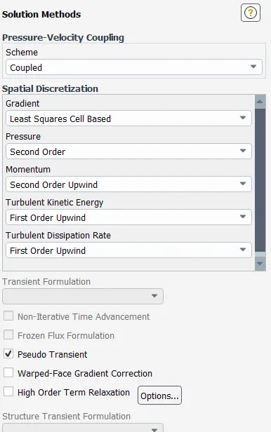
4. Solution

For the Solution Residuals Monitor, the Magnitude was changed to 1e-6 to get more accuracy.

Hybrid Intilizization was used in order to initialize this simulation.

As this was Steady-State Simulation so the Simulation was run for 250 cycles and the results were generated easily.

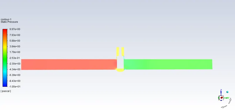
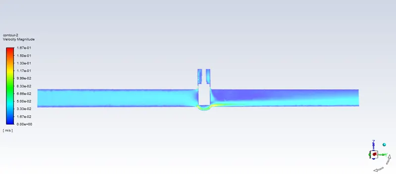
Case Study 1: When the Valve lift is set to 20mm.

Pressure Contour

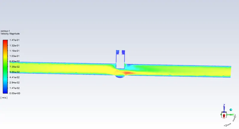
Velocity Contour

Mass Flow Rate

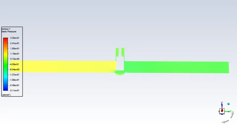
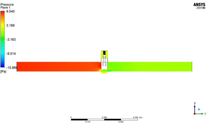
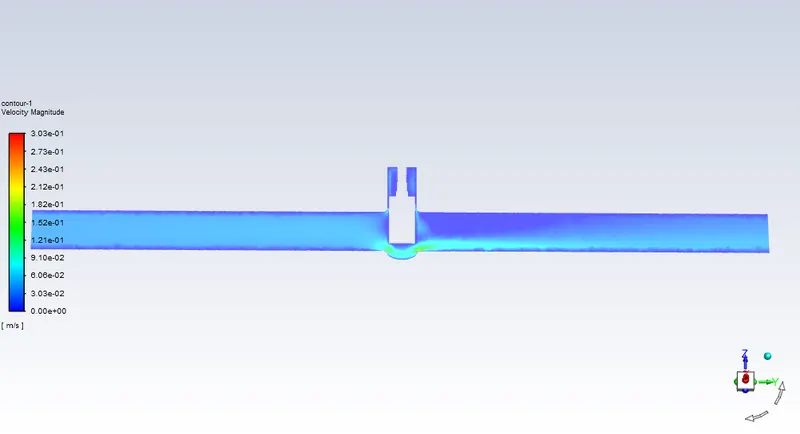
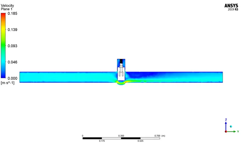
Case Study 2: When the Valve lift is set to 30mm.

Pressure Contour

Velocity Contour

Case Study 3: When the Valve lift is set to 40mm.

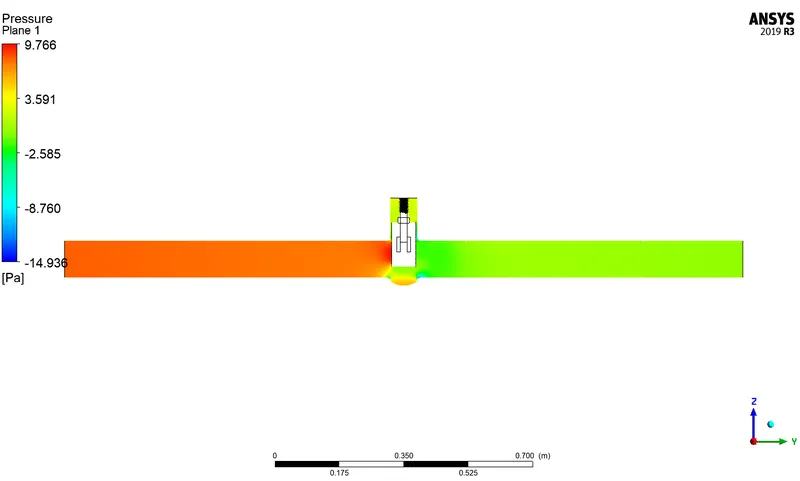
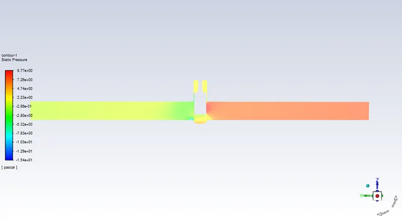
Pressure Contour

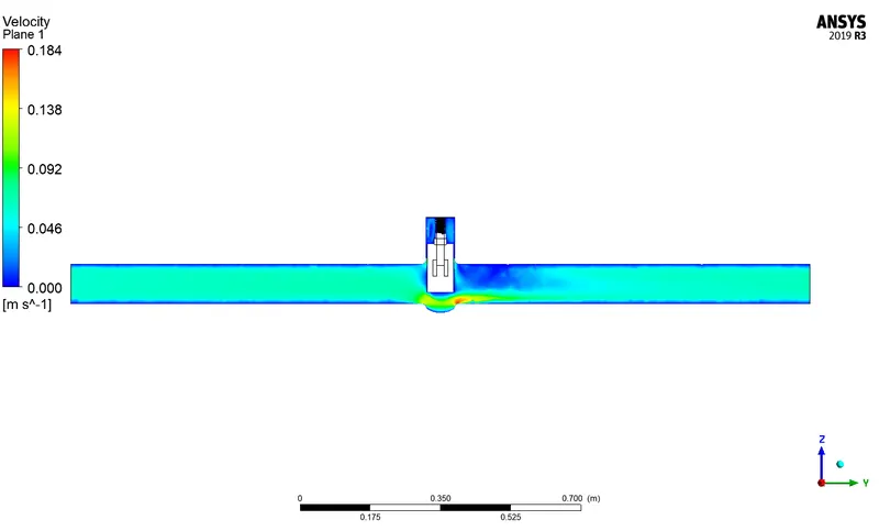
Velocity Contour

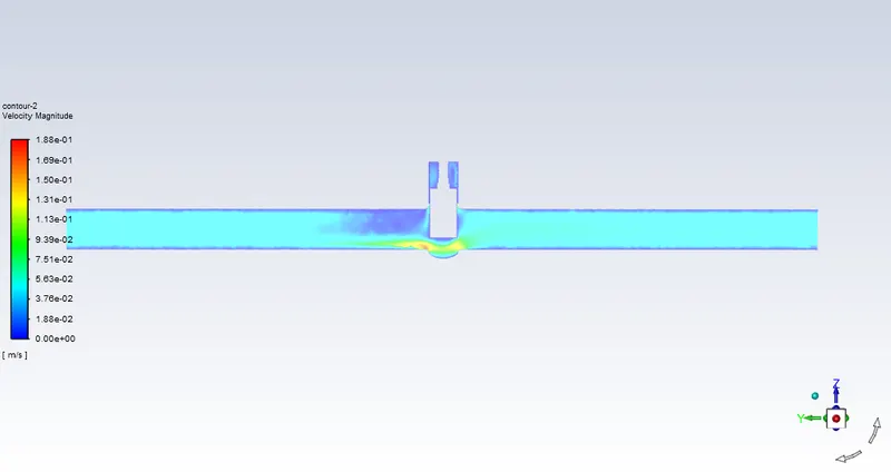
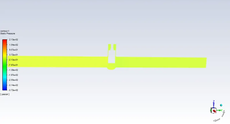
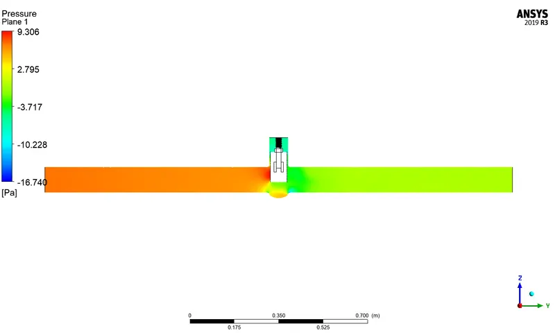
Case Study 4: When the Valve lift is set to 50mm.

Pressure Contour

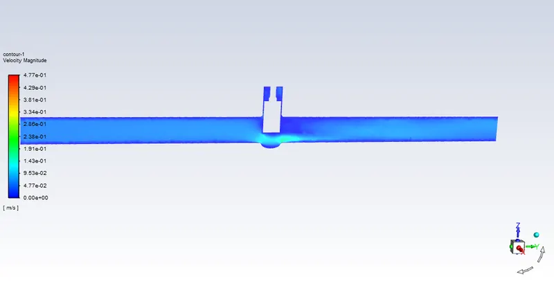
Velocity Contour

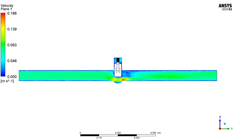
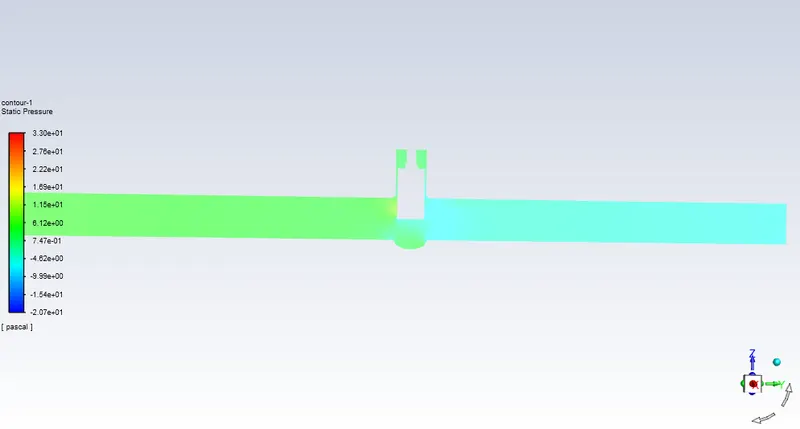
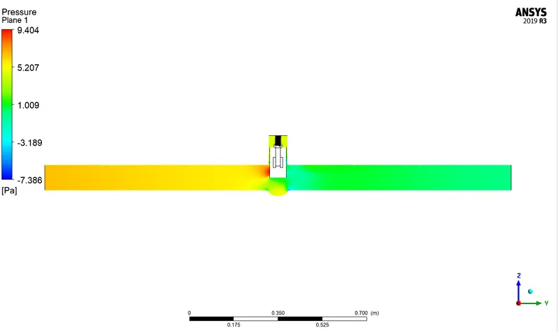
Case Study 5: When the Valve lift is set to 60mm.

Pressure Contour

Velocity Contour

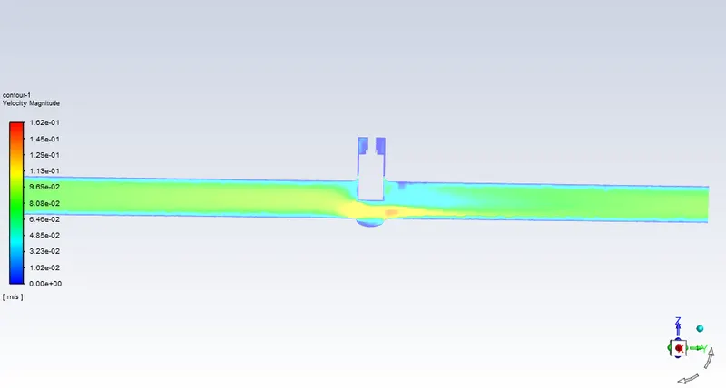
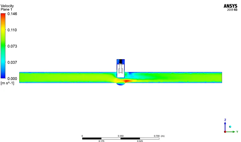
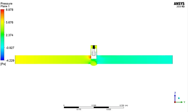
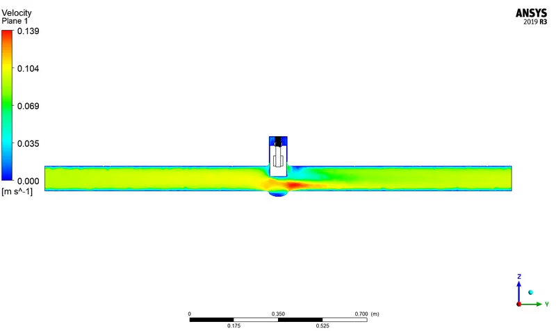
Case Study 6: When the Valve lift is set to 70mm.

Pressure Contour

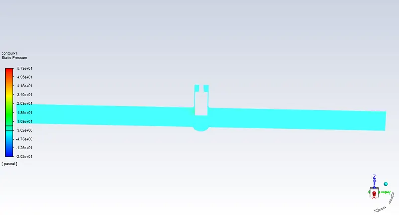
Velocity Contour

Conclusion

The Flow Coefficient of a device is a reltive measure of its efficiency at allowing fluid flow. It describes the relationship b/w the pressure drop acroos the tube length through orifice and the flow rate.

it can be represented by

`C_v=Qsqrt((SG)/(Pressure Drop))`

Where

Q is rate of flow (Gallons/minutes)

SG is the specific gravity of water(SG=1)

Pressure Drop is the pressure drop across the length of device.(Psi)

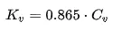
The metric equivalent flow factor (K_v; commonly used everywhere else in the world with the exception of the United States) is calculated using metric units :

`K_v=Qsqrt((SG)/(Pressure Drop))`

Q is rate of flow (m^3/h)

SG is the specific gravity of water(SG=1)

Pressure Drop is the pressure drop across the length of device.(bar)

Valve Position (mm)	Inlet Mass Flow (Kg/s)	Outlet Mass Flow (Kg/s)	Inlet Average Pressure (Pa)	Outlet Average Pressure (Pa)	Pressure Drop(Pa)	Flow Rate`m^3/h`
20	0.02398	0.23989	10	0.4747	9.5252	0.8636
30	0.36508	0.36552	10	1.0783	8.9216	1.3158
40	0.47610	0.47608	10	1.8760	8.1239	1.7138
50	0.56642	0.56618	10	2.6517	7.3482	2.0382
60	0.67965	0.67907	10	3.7071	6.2928	2.4446
70	0.77321	0.78006	10	5.1585	4.8413	2.8082

Valve Position(mm)	Pressure Drop (bars)	Pressure Drop(Psi)	Flow Coefficient `C_v`	Flow Factor `K_v`	`K_v/C_v`
20	9.525e-5	0.0013815	`C_v=Qsqrt((SG)/(Pressure Drop))` `C_v=4.4*0.863sqrt((1)/(0.001381))=102.23`	88.48	0.865542
30	8.9216e-5	0.0012939	`C_v=Qsqrt((SG)/(Pressure Drop))` `C_v=4.4*1.3158sqrt((1)/(0.001293))=160.95`	139.31	0.865542
40	8.1239e-5	0.0011782	`C_v=Qsqrt((SG)/(Pressure Drop))` `C_v=4.4*1.7138sqrt((1)/(0.001178))=219.691`	190.15	0.865542
50	7.3482e-5	0.0010657	`C_v=Qsqrt((SG)/(Pressure Drop))` `C_v=4.4*2.0382sqrt((1)/(0.0010657))=274.7112`	237.77	0.865542
60	6.2928e-5	0.0009126	`C_v=Qsqrt((SG)/(Pressure Drop))` `C_v=4.4*2.446sqrt((1)/(0.0009126))=356.046`	308.14	0.865542
70	4.8414e-3	0.0007021	`C_v=Qsqrt((SG)/(Pressure Drop))` `C_v=4.4*2.8082sqrt((1)/(0.0007021))=466.29`	403.59	0.865542

The Parametric study of the gate valve indicated that if the valve lift is increases the mass flow rate is also increases at the outlet.

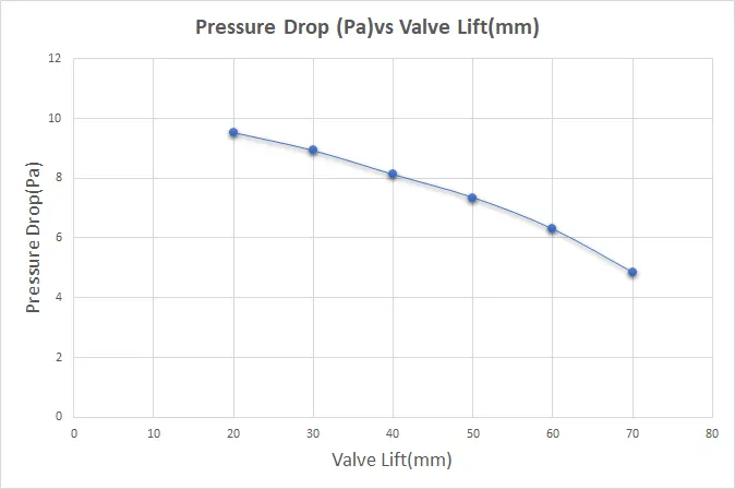
Pressure drop decreases as the valve lift increases whereas the outlet velocity increases.

Parametric Study Makes work easier by automating everything.