Flow Simulation over Cylinder using ANSYS

Aim:

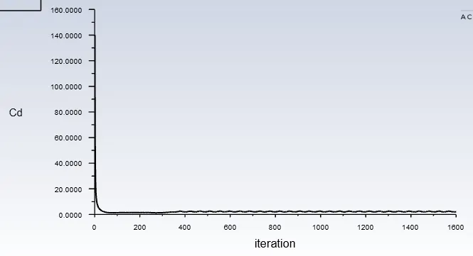
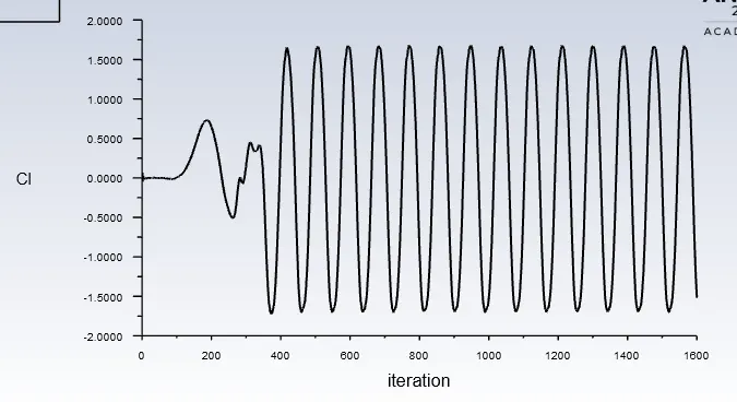
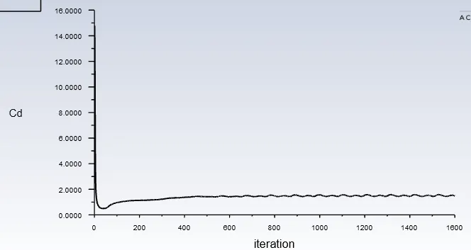
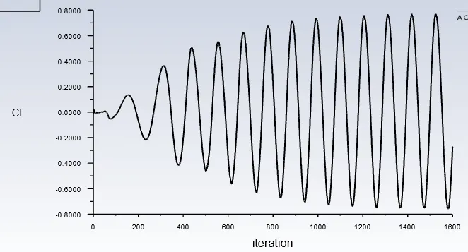
The Major Objective of this project was to simulate the flow over the circular cylinder using Ansys fluent and Study the Phenomenon of Karman Vortex along with an estimation of the Coefficient of Lift `C_l` and Drag `C_d` over the cylinder for various Reynolds Number ie. 10,100,1000,10000, & 100000.

Introduction

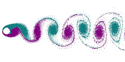
The flow characteristics over a cylinder are one of the most applicable important topics of research. The cylinder subjected to low Reynolds number experiences flow separation, and oscillations in the wake region. The periodic nature of the vortex shedding phenomenon can sometimes result in unwanted structural vibrations, which leads to structural damage. A Von Karman vortex is a repeating pattern of swirling vortices arising in the wake of the flows around the cylinder. This process can be only seen at a particular critical Reynolds number.

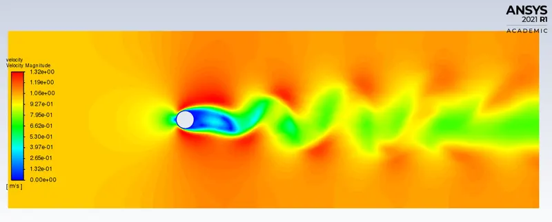
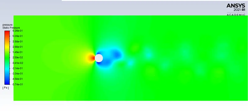
These Vortices are created at the back of the body and they detach randomly from either side of the body. The fluid flow past the object creates alternating low-pressure vortices or eddies on the downstream side of the object. The object will tend to move towards the low-pressure zone and flow separation occurs results in a vortex generally found at Re above 40 but can be clearly seen at Re 100.

This Project contains the following:

Case Study 1

• Transient and Steady-State Simulation over the Cylinder at Reynold number 100 and Estimation of Strouhal number.

Case Study 2

• Estimation of `C_d " & " C_l` for various Reynolds number ie. 10,100,1000,10000, & 100000.
• Study the effect of Re on the coefficient of Drag.

STEADY STATE SIMULATION:

These are the simulation we run if are just interested in the end result and not in how those results are getting formed with time. The properties do not change with respect to time or there are no time derivative terms in the equations of motion that govern the fluid flow.

If we want to see how results are changing w.r.t time and how the solution is getting formed over time then we need to run the TRANSIENT STATE SIMULATION.

The time is in Cycles for STEADY STATE SIMULATION whereas time is in Seconds for TRANSIENT STATE SIMULATION.

Reynold Number is the ratio of Inertial force to the Viscous force

`"Re"=( rhoVD)/mu`

1.Geometry Creation

First of all, The Cylindrical shape along with domain body geometry was created using a separate CAD package i.e. Solidworks. Then the same geometry was imported in Ansys workbench for generating the fluid flow domain volume to define the boundary conditions and further proceed with Pre Processing, and post-processing the results.

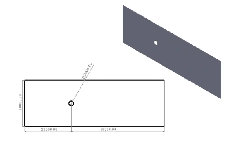
Image 1: CAD model of Geometry

2.Boundary Creation and Meshing

After the control volumes or the fluid flow domain are perfectly created the boundary tags were created in order to assign the different boundary conditions ie. velocity, temperature (If needed), or some other physics. For this geometry, 4 different boundary tags or names were created that were used earlier to assign the boundary condition. The four names are Inlet, Cylinder Wall, Outlet, and Symmetry Walls.

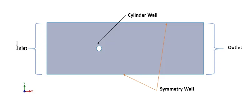
Image 2: Geometry representing the various boundary Tags.

Meshing

As the Geometry has flow simulation so for that many points were assumed before creating the mesh in order to capture the flow around the cylinder properly. The triangular mesh elements were chosen in order to make it more fine along with various inflation layers around the cylinder to capture the von Karman vortex carefully.

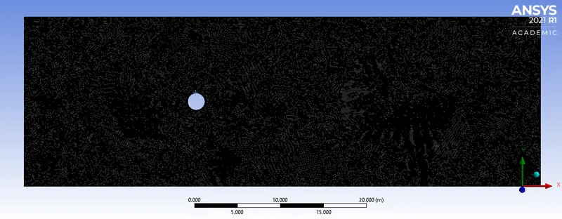
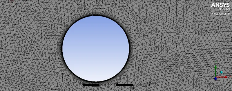
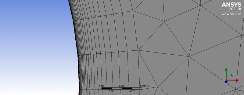
Image 3: Representation of A)Triangular Shape elements, B) 36 Number of Divisions near the walls of the cylinder, and C) 25 Inflation layers with the growth rate of 1.2

All Triangle Method was used to create the Triangular Shaped Mesh Elements

Elements Size=0.1m

Edge Sizing was created near to cylinder wall to increase the 36 number of divisions near the wall to capture the flow properly.

25 Inflation layers were added in order to make more refined mesh near walls of a cylinder with a growth rate of 1.2

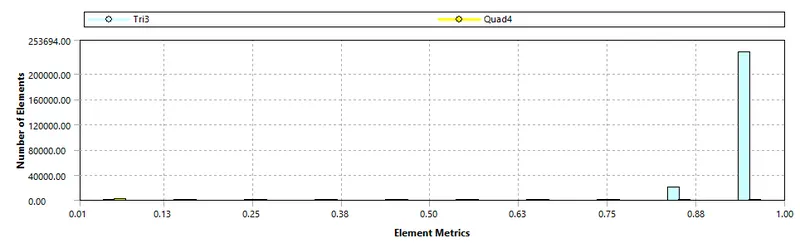
3. Case Study Setup

For setting up the case study Ansys Fluent was used in order to simulate the case study.

The various parameter was considered while setup this case study. The case study setup dock was used to set up the problem which appears on the left-hand side of the converge studio

S.No.
1	Models	Viscous Model-`-Laminar for low RE Viscous Model-`-K-Omega SST	Two different viscous models were chosen for different ranges of Reynolds numbers.
2	Material	Air (N2:O2::23%:77%)	Air was used as the fluid inside the Flow over cylinder case study
3	Cell Zone Condition	Control Volume Region was set to Air	The flow inside the Control volume wanted it to be only air with Different Properties to alter the Reynolds number.
4	Boundary Conditions	Inlet Velocity 1m/s
		Outlet Zero gauge pressure
		Cylinder wall No-slip(Velocity near the wall is Zero)
		Top and Bottom Wall- Symmetry Wall

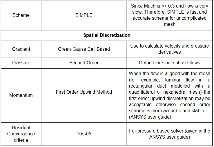
Scheme Used

4. Solution

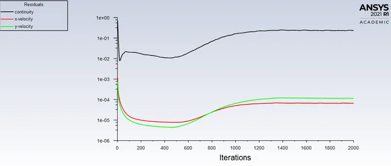
For the Solution Residuals Monitor, the Magnitude was changed to 1e-6 to get less error with more accuracy.

The Surface Report for Velocity With the monitor point behind the cylinder was used to generate the report that can be used to determine the frequency of Vortex behind the cylinder.

Hybrid Intilizization was used in order to initialize this simulation.

Steady-State Simulation and Transient Simulation were performed to achieve more realistic results and vortex visualization behind the cylinder.

Case Study 1

Steady-State Simulation

Reynold Number 100

Residuals Plots

Velocity Monitor Point plot

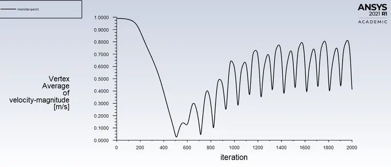
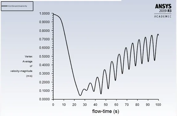
The wavy pattern can be seen because we have placed a monitor point behind the Cylinder that will keep track of the velocity which can be used to find the frequency of oscillation to find the Strohual number. The oscillation is due to the formation of Von Karman Vortices behind the cylinder at a Reynolds number of 100.

Velocity Contour

Pressure Contour

Case Study 1

Transient Simulation Simulation

Reynold Number 100

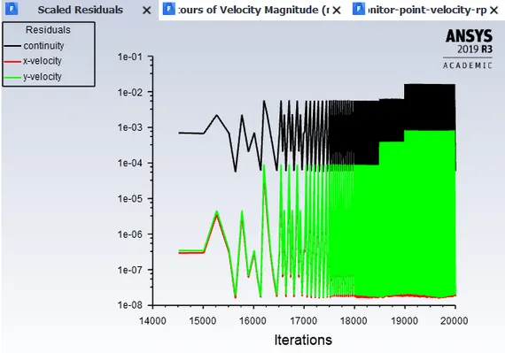
Residuals Plots

Velocity Monitor Plot

The Strouhal number is a dimensionless number that represents the ratio of inertial force due to the Local Acceleration of the flow to the inertial forces due to the convective acceleration.

`S_(tr)=(fL)/U`

f is the Frequency of the Oscillations(1/s)

L is the Characteristic length of the body(m)

U is the Flow Velocity(m/s)

Calculation of Strouhal Number

Cylinder Diameter=2m

Inlet Velocity=1m/s

Frequency=No of Ossicilation/Time=`7.5/50=0.15`

`S_(tr)=f*d/v=0.15*2/1=0.3`

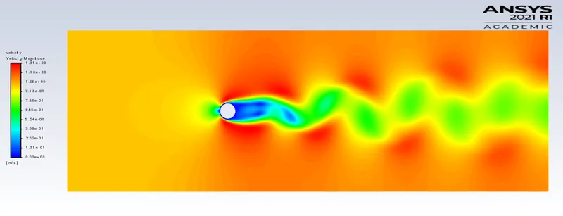
Velocity Contour

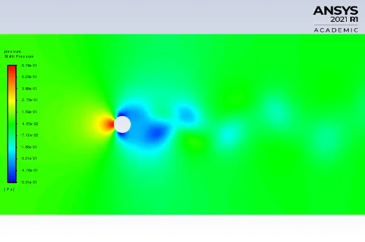
Pressure Contour

Case Study 2: Study the Coefficient of Lift and Drag over the Cylinder when the Reynolds number is changed

For this case, In order to change the Reynolds number, we will be changing the density of air to change the Reynolds Number.

The following cases have been studied.

S.No.	Reynolds Number	Viscosity
1	10	0.2
2	100	0.02
3	1000	0.002
4	10000	0.0002
5	100000	0.00002

For Calculation of `mu`

V=1m/s

Density=1 kg/m^3

Diamter of Cylinder =2m

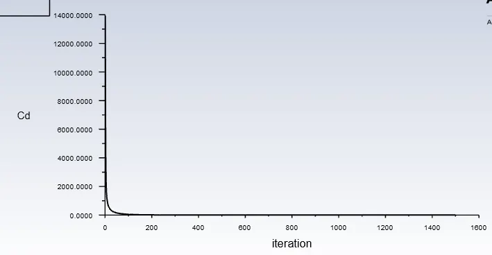
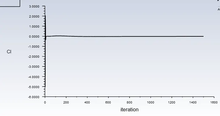
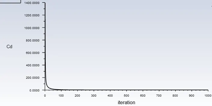
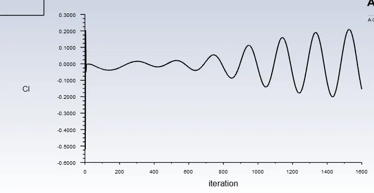
All the results were generated using Steady-State Simulation for 1000 Iteration

	Reynolds Number=10
Coefficient of Drag 0.021
Coefficient of Lift 0.002888
Velocity Contour

	Reynolds Number=100
Coefficient of Drag 1.389
Coefficient of Lift 0.19
Velocity Contour

	Reynolds Number=1000
Coefficient of Drag 1.226
Coefficient of Lift 1.75
Velocity Contour

	Reynolds Number=10000
Coefficient of Drag 1.4
Coefficient of Lift 0.7
Velocity Contour

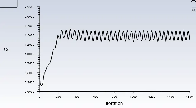
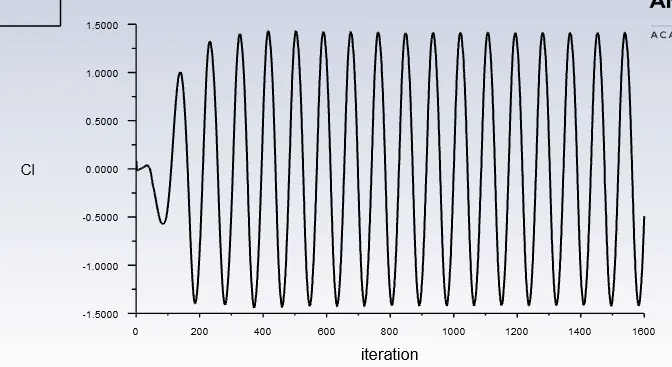
	Reynolds Number=100000
Coefficient of Drag 1.65
Coefficient of Lift 1.45
Velocity Contour

Conclusion

1. Vortex shedding can be easily seen in the case of both Steady State and Transient Simulation. But Transient Simulation produces better results and more Realistic.
2. Strouhal Number calculation is only possible in the case of Transient simulation as the frequency changes with respect to time.
3. As the Reynolds number Increases, The drag Coefficient also Increases.
4. Drag force is inversely proportional to Reynolds number(Re<300 where the flow is laminar after that it gets converted to turbulent) on changing the viscosity.
5. Vortex shedding can be observed after Re 40 .