Project

CFD Simulation of Port-Fuel-Injection Engine using Converge CFD

AAntim Gupta25 Jan 2022

Aim:

The Main objective of this project was to setup Full-hydrodynamics solver transient simulation of a port fuel injection engine using converge CFD.

Introduction

Port injection, the fuel injectors are positioned on the air intake leading to each cylinder of your engine. As your engine sucks in air to later be compressed your fuel injectors will spray a fine mist of fuel that will eventually mix with the ambient air as it gets sucked into your engine.

This allows the air and fuel enough time to mix with each other as they are eventually sucked into the cylinder wall. That air and fuel mixture would then be compressed and then ignited to complete the combustion process of your engine.

Port injection is the other of the two injection technologies and has been around for quite some time.

Benifits of PFI Engine

Since the 1980s, when carburetors were supplanted as the primary fuel injection technology, port injection has been in use. Fuel is injected into your air intake port and drawn into the piston, providing fuel for your engine's combustion stroke.

The advantage of port injection is that it allows air to uniformly mix with the gasoline before it is supplied into the engine cylinder. When the air and fuel mixture is evenly mixed, the combustion process can burn all of the fuel fed into the engine cylinder, which reduces carbon buildup from unburned fuel.

Direct injection allows less time for the fuel to mix with the air entering the cylinder, which can result in hot spots forming inside the engine cylinder. Hot spots are bad because they can cause one place to become significantly hotter than the rest of the engine cylinder walls, rather than uniformly heating them.

STEADY STATE SIMULATION:

These are the simulation we run if are just interested in the end result and not in how those results are getting formed with time. The properties do not change with respect to time or there are no time derivative terms in the equations of motion that govern the fluid flow.

If we want to see how results are changing w.r.t time and how the solution is getting formed over time then we need to run the TRANSIENT STATE SIMULATION.

The time is in Cycles for STEADY STATE SIMULATION whereas time is in Seconds for TRANSIENT STATE SIMULATION.

-------------------------------------------------------------------------------------------------------------------------------------------------------

The project mainly focuses on the following things:-

1. Importing the(.Stl) file on Converge Studio then cleaning up the geometry removing the intersection, patching the new open edge, deleting the unwanted edge, and Fixing the normal orientation of the geometry.

2. Creating Virtual Wind Tunnel using proper Dimension.

3. Case Setup using Converge Studio using proper Solver and Boundary Conditions.

4. Solving the Case Study Files using Cygwin.

5. Post-Processing the result Using ParaView generating plots, contours

1. Importing the Geometry for Geometry Clean Up using Converge Studio and BOundary Flagging

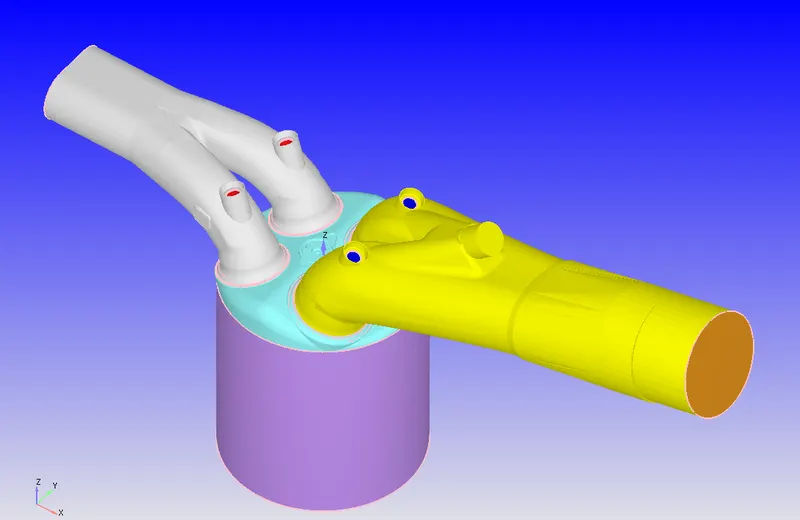
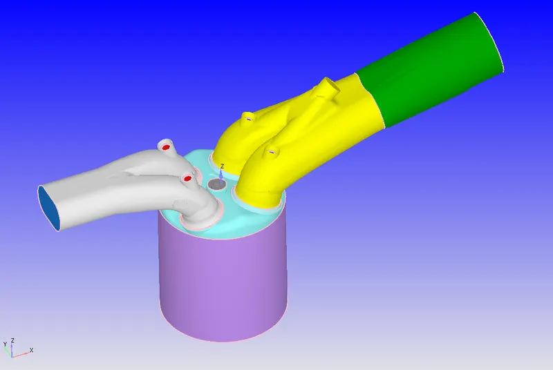
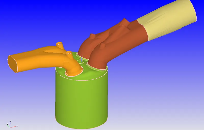
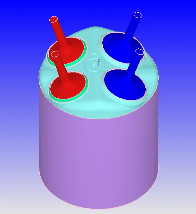
Firstly the Geometry(.stl) was imported in Converge Studio. The diagnostic tool was used to find the open edge, Intersection edges, and other errors like orientation error. Many features were used to repair the geometry like 1. Deleting the edge, node, face. 2. Patching the edge using the patch tool. 3. Stitching the two misalign edges.

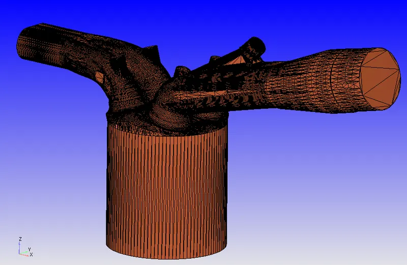
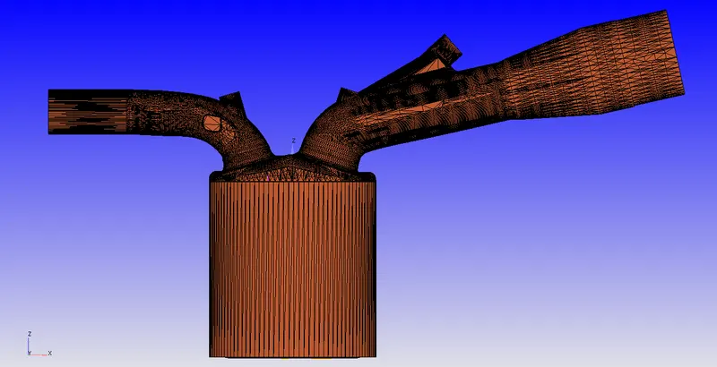
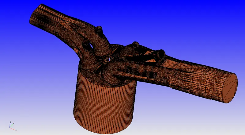
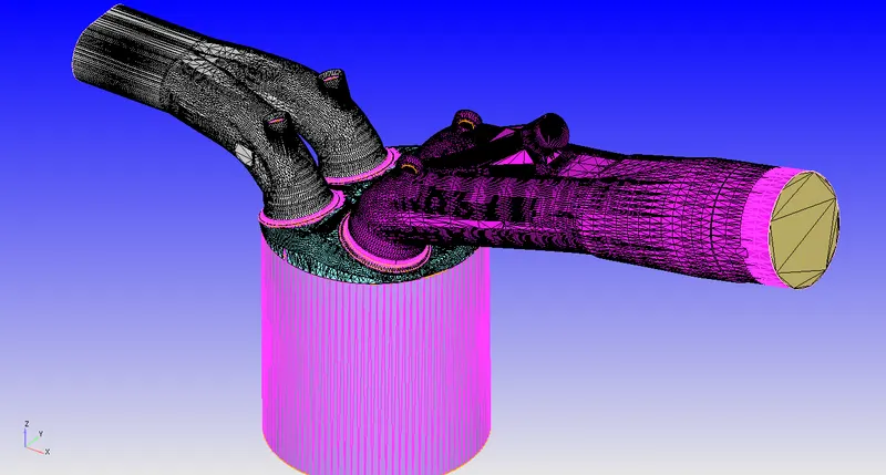
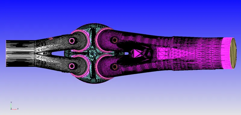
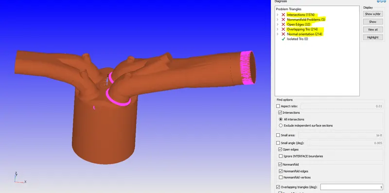
The car geometry that was provided had 32 total open edge errors, 1574 intersection. so geometry cleaning plays an important role in setting up a simulation of a engine There were many features that were used to clean the geometry. First, the geometry was checked using the Diagnostic tool to check what kind of error is present then our main target was to repair an open edge without forming an intersection.

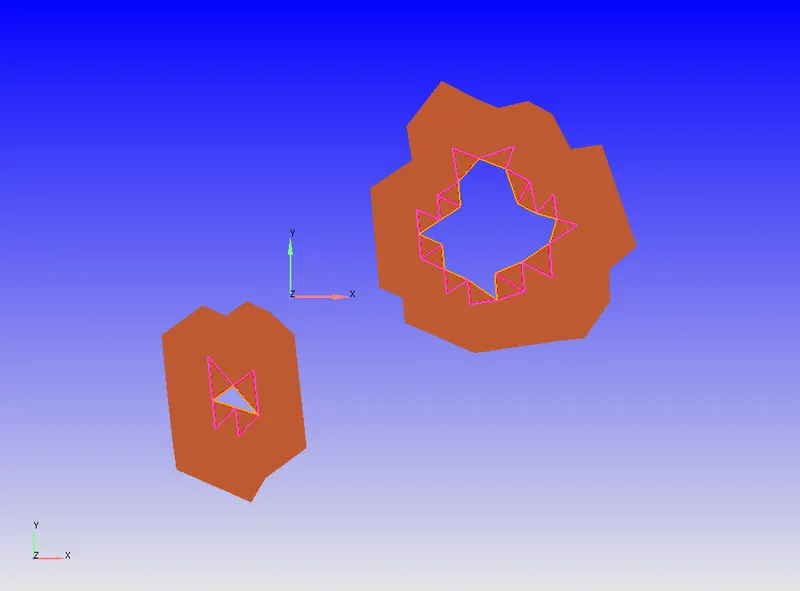
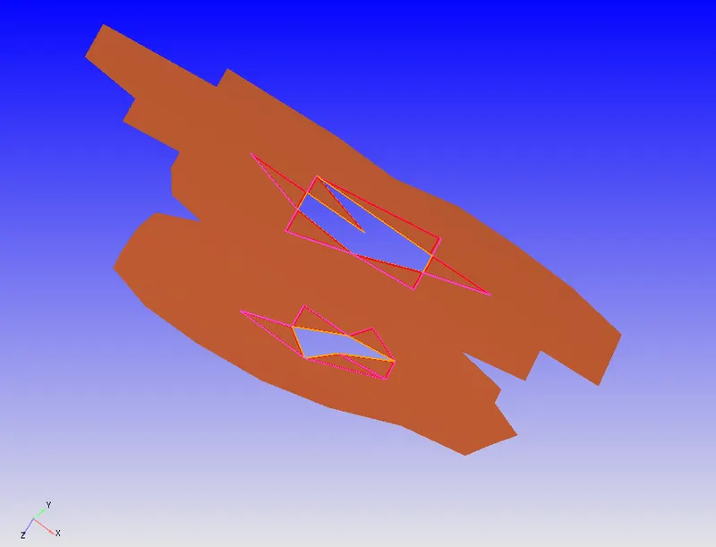
First, the surface(Triangle) was deleted shown in green color then the extra edges were removed to make a perfect open loop that can be patch letter. For patching those new open edge the edges were checked and patch repair option was used to patch the open edge method. Then the geometry was checked again to find any error.


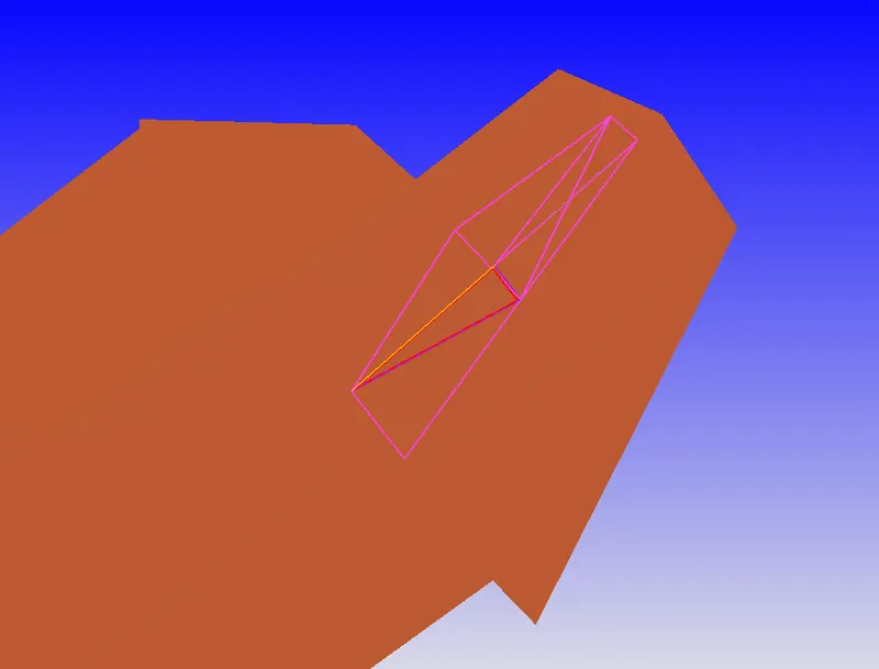Open Edges in the piston wall	Open Edges in the Inflow duct	Intersection error

The bpoundary fencing feature was used to mark the fencing in the geomtery and Boundary flagging was done after that selecting the proper number of triangle surfaces. Total 17 Boundary Tags were created in order to define region and physics for engine simulation.

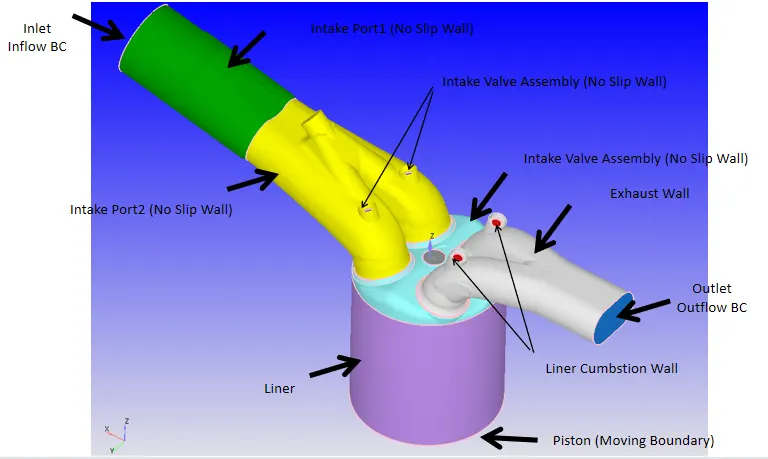
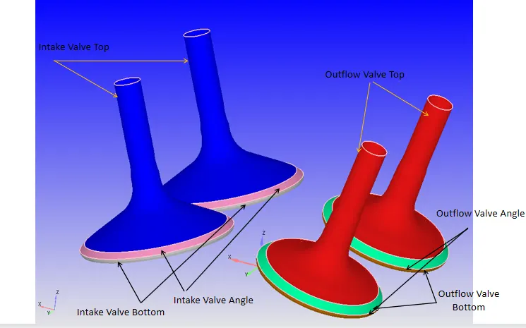
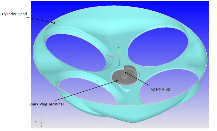
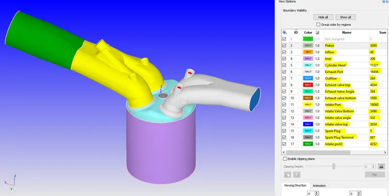
Geomtery of IC Engine was flagged with boundary names represented in above picture along with boundary ID and sum of triangle the particular boundary is created from.

The normal orientation was fixed using automatic option present in Transform>Normal> Automatic fix all the normals.

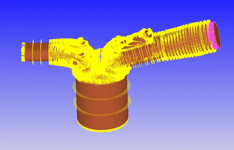
Normal poitning outward

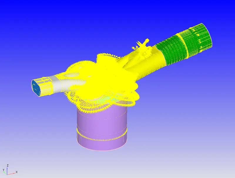
After transforming the Normals inside geometry

After doing Geometry clean up, The geometry was again finally checked for any error using the Diagnostic tool. At last, all the all errors were repaired as shown in the above picture.

Geometry was finally Cleaned and can be used for further pre processing.

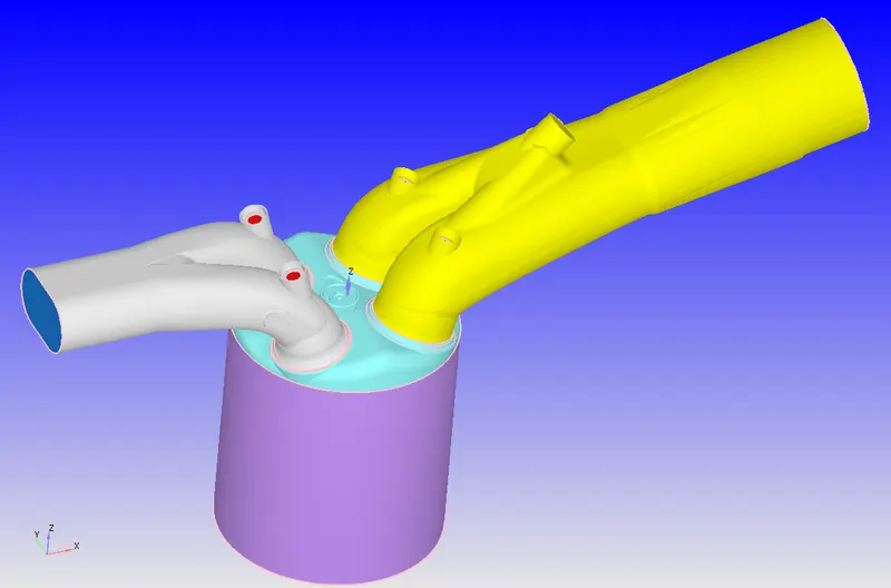
The Geometry with Error can be downloaded from here: Geometry

2.Case-Study Setup

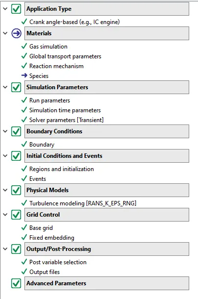
The various parameter was considered while setup this case study. The case study setup dock was used to set up the problem which appears on the right-hand side of the converge studio.

2.1 Application Type:

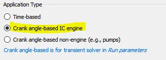
In order to run a steady-state simulation, firstly, under the Application type in the setup tree, a "Crank angle based IC engine" simulation must be selected.

2.2 Materials:

Under the material tab "Gas simulation" was selected and "Air" as a predefined mixture.

Gas: Air

Global Transport Parameters: Fixed value

by default, the following value is considered.

Prandtl Number : 0.9

Schmidt Number : 0.78

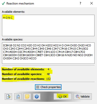
Reaction Mechanism was enabled and the file file was uploaded

3.3 Simulation Parameters

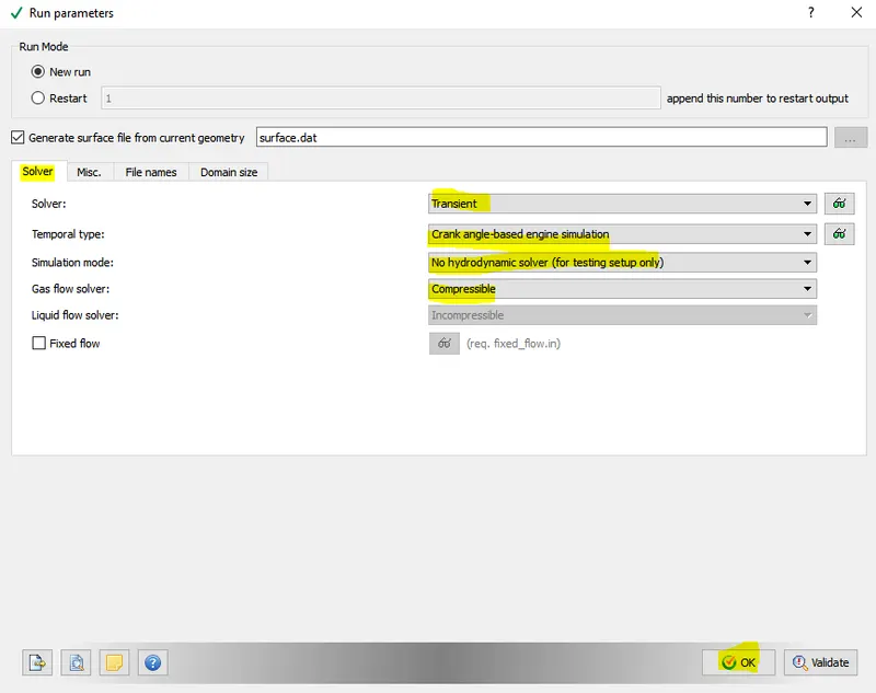
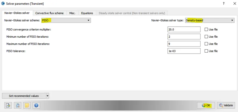
The Transient solver was selected for running this case study along with a "Density-based" solver.

2.4: Boundary Conditions

In this tab, The volumetric region and physics for each boundary were defined.

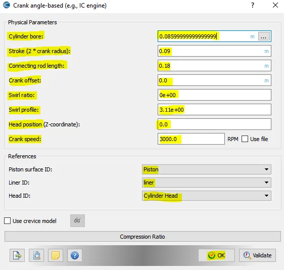
Engine Geometric Parameters

Bore =0.086 m
Stroke = 0.09 m
Connecting rod length = 0.18 m
RPM = 3000

Run parameters

Simulation mode: No Hydro

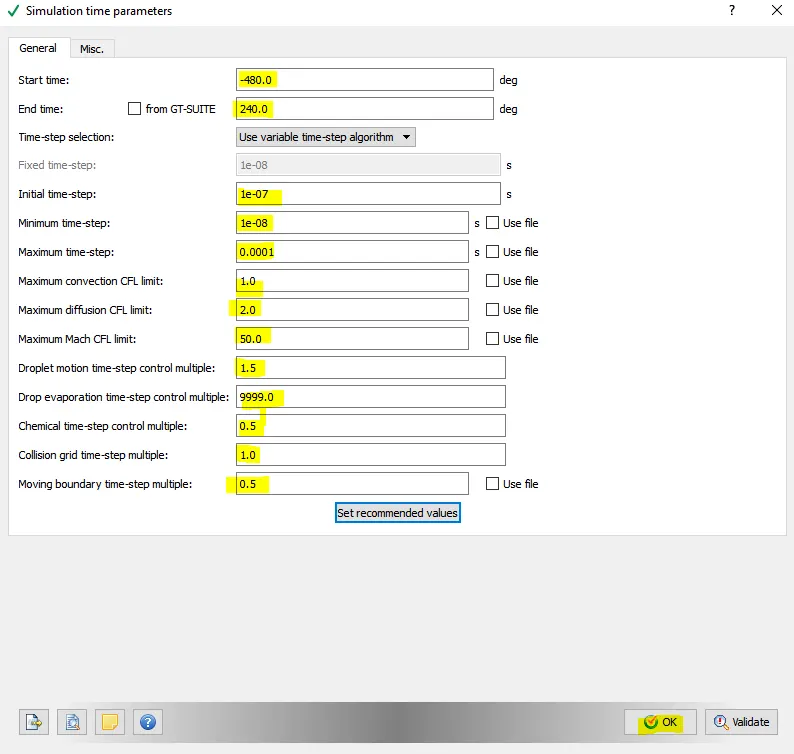
Simulation time parameters

Start time : -480 deg
end time : 240 deg

Boundary conditions

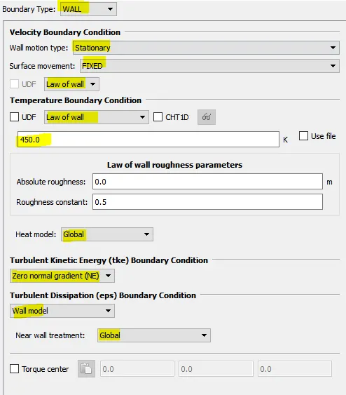
Piston temperature - 450K
Liner temperature - 450K
Head temperature - 450K
Spark Plug temperature - 450K
Spark Plug electrode temperature - 600K
Exhaust ports temperature - 500K
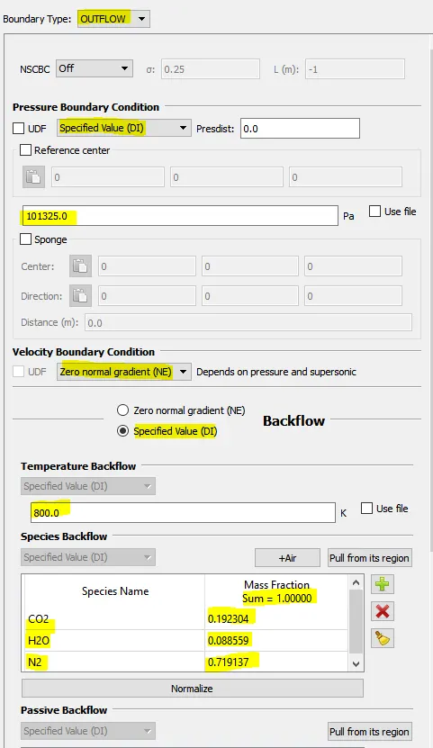
Exhaut outflow - 1 bar
Exhaust outlflow temperature - 800k
Exhaust species concentration - Calculated using the stoichiometric condition
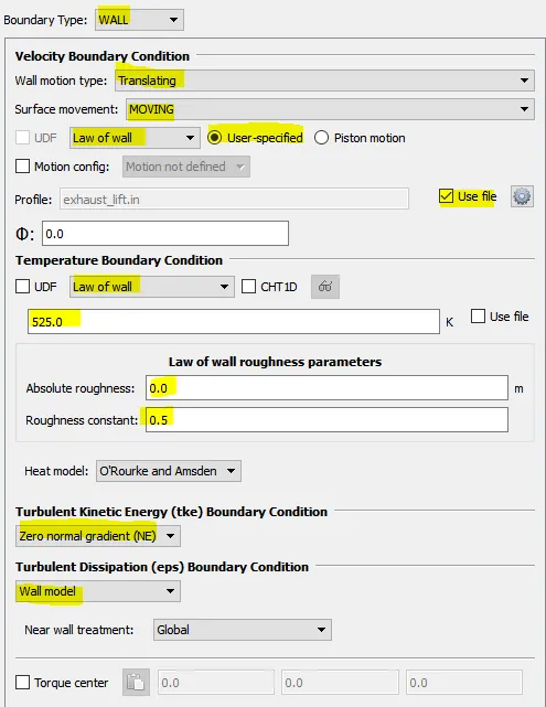
Exhaust valve top temperature - 525K
Exhaust valve angle temperature - 525K
Exhaust valve bottom temeprature - 525K
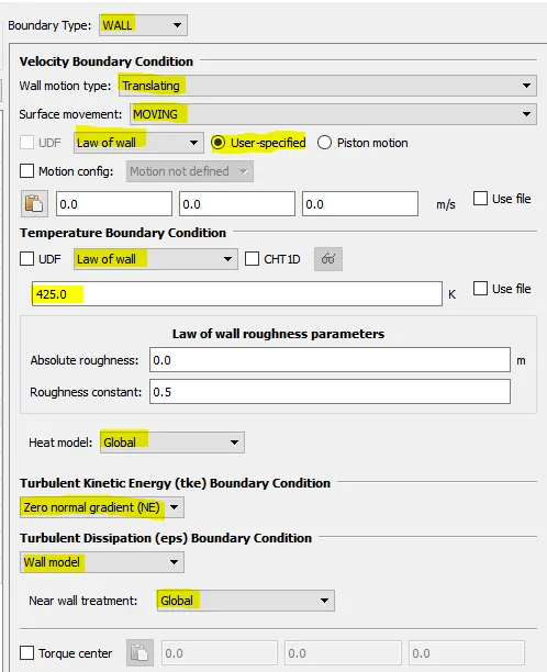
Intake port - 1 temperature 425K
Intake port - 2 temperature 425K
Inflow pressure - 1 bar total pressure
Inflow temperature - 363K
Inflow species - Air
Intake valve top temperature - 480K
Intake valve angle temperature - 480K
Intake valve bottom temeprature - 480K

Initial conditions

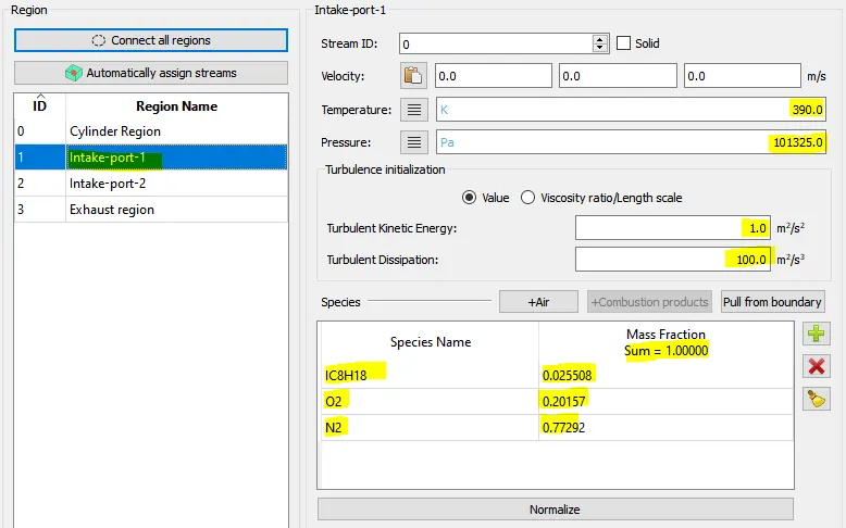
Intake port - 1 (closer to combustion chamber)
- ic8h18 - 0.025508
- o2 - 0.20157
- n2 - 0.77292
- Temperature - 390k
- pressure - 1 bar
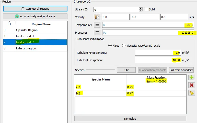
Intake port - 2 (away from combustion chamber)
- Air
- Temperature - 370K
- Pressure - 1 bar
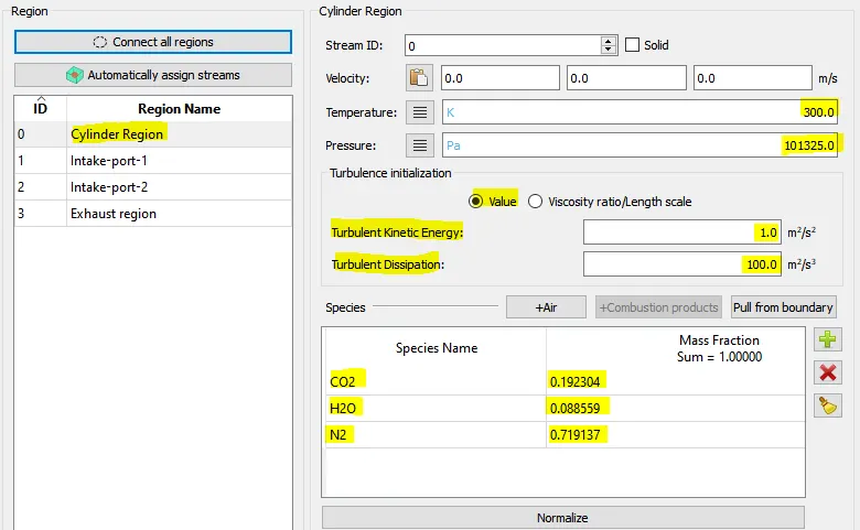
Cylinder
- Pressure - 1.85731 bar
- Temperature - 1360K
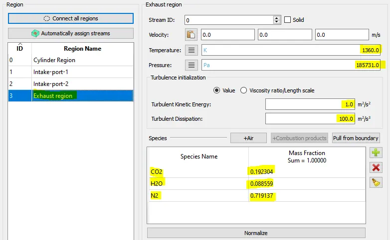
- Stoichiometric composition

STIOCHIOMETRIC Calculations

Species	Moles	Molecular weight(g/mol)	Mass	Mass Fraction
Co2	8	44.01	352.08	0.192304
H2O	9	18.01528	162.1375	0.088559
N2	47	28.0134	1316.63	0.719137
Total

Combustion Physics Setup.

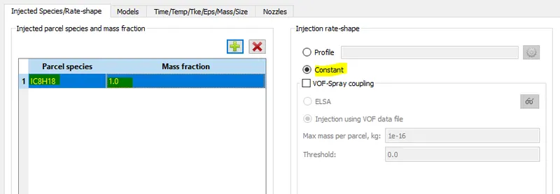
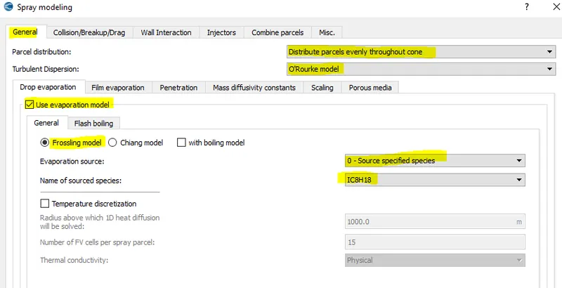
Spray Modelling

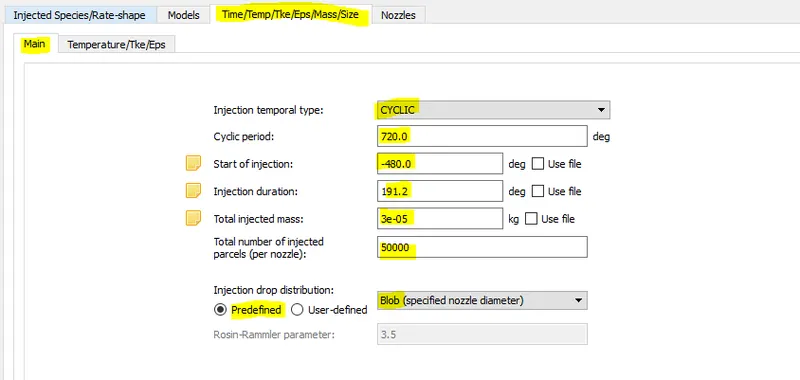
Injection Parameters

Fuel flow rate = 7.5e-4 Kg/second
Injection start time = -480.0
Injection duration = 191.2
Fuel temperature = 330K

Nozzle positions

Nozzle diameter = 250 micro-meter

Circular injection radius = Nozzle radius

Spray cone angle = 10

Nozzle 0
- center 0.0823357 0.00100001 0.07019
- Align Vector -0.732501 0.210489 -0.647408
Nozzle 1
- center 0.0823357 -0.00099999 0.07019
- Align Vector -0.732501 -0.210489 -0.647408
Nozzle 2
- center 0.0823357 -0.0004 0.07019
- Align Vector -0.5 -0.2 -0.647408
Nozzle 3
- center 0.0823357 0.0003 0.07019
- Align Vector -0.5 0.2 -0.647408

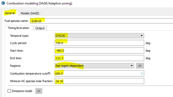
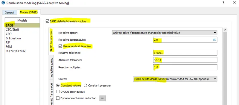
Spark Ignition Parameters

Start of spark = -15 deg
Spark duration = 10 deg
Spark location = -0.003 0 0.0091
Spark radius = 0.0005m

Boundary_Name	Boundary_Type	Paramter_Defined	Region	Boundary ID
1. Piston	Wall		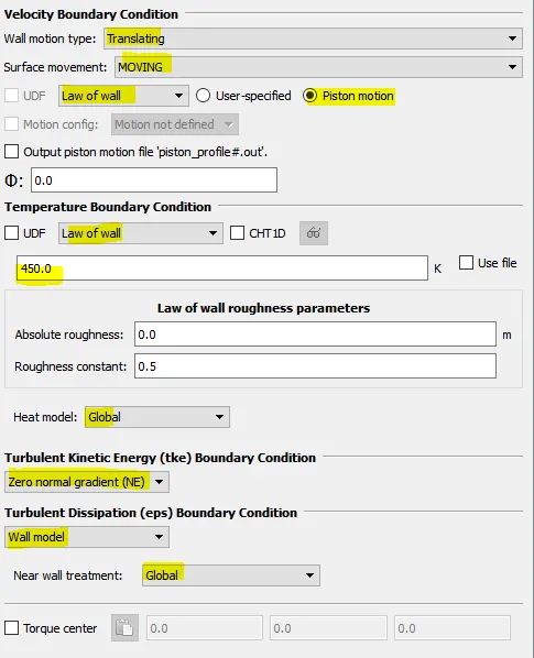Cylinder Region	1
2. Inflow	Inflow BC		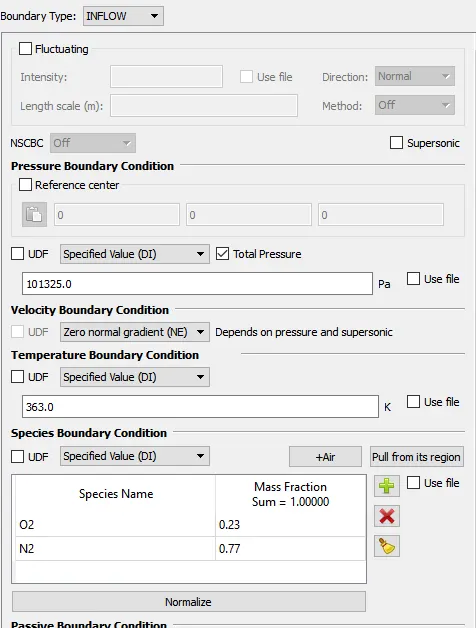Intake Port-2	2
3. Liner	Wall		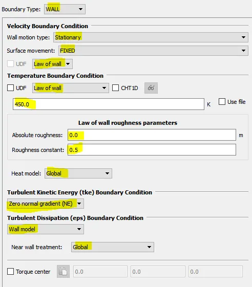Cylinder Region	3
4. Cylinder Head	Wall		Cylinder Region	4
5. Exhaust Port	Wall		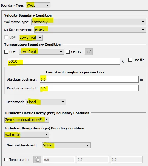Exhaust Region	5
6. Outflow	Outflow		Exhaust Region	6
7. Exhaust Valve Top	Wall		Exhaust Region	7
8. Exhaust Valve Angle	Wall		Exhaust Region	8
9. Exhaust Valve Bottom	Wall		Exhaust Region	9
10. Intake port	Wall		Intake Port-1	10
11.Intake Valve Bottom	Wall		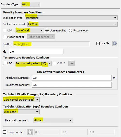Cylinder Region	11
12. Intake Valve Angle	Wall		intake port1	12
13. Intake Valve Top	Wall		intake port1	13
14. Spark Plug	wall		Culinder Region	14
15. Spark plug Terminal	wall		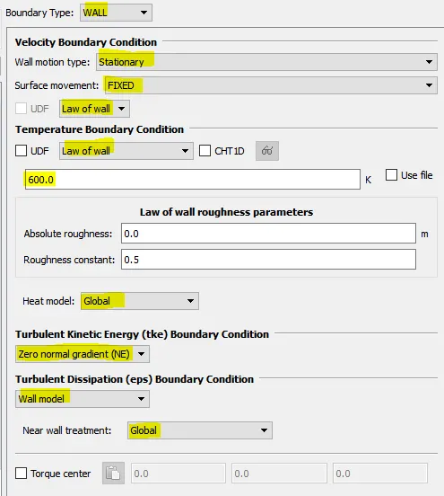Cylinder Region	15
16. Intake port2	Wall		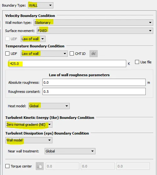Intake port2	16

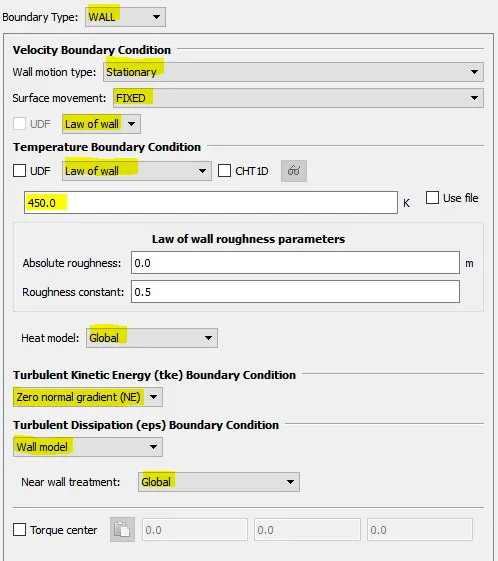
2.5: Initial Conditions and Events

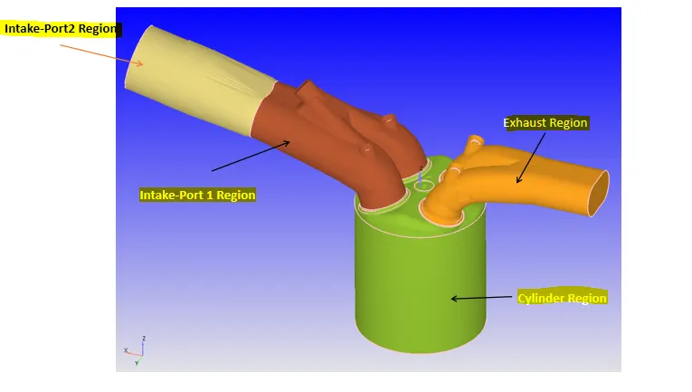
4 Volumetric Region was created in order to assign this to all the boundary tag.

Different Volumetric Regions are:-

1. Cyliner Region

Intake Port-1 Region

Intake- port-2 Region

Exhaust Region

Boundary Flagging according to regions

2.6: Physical Models

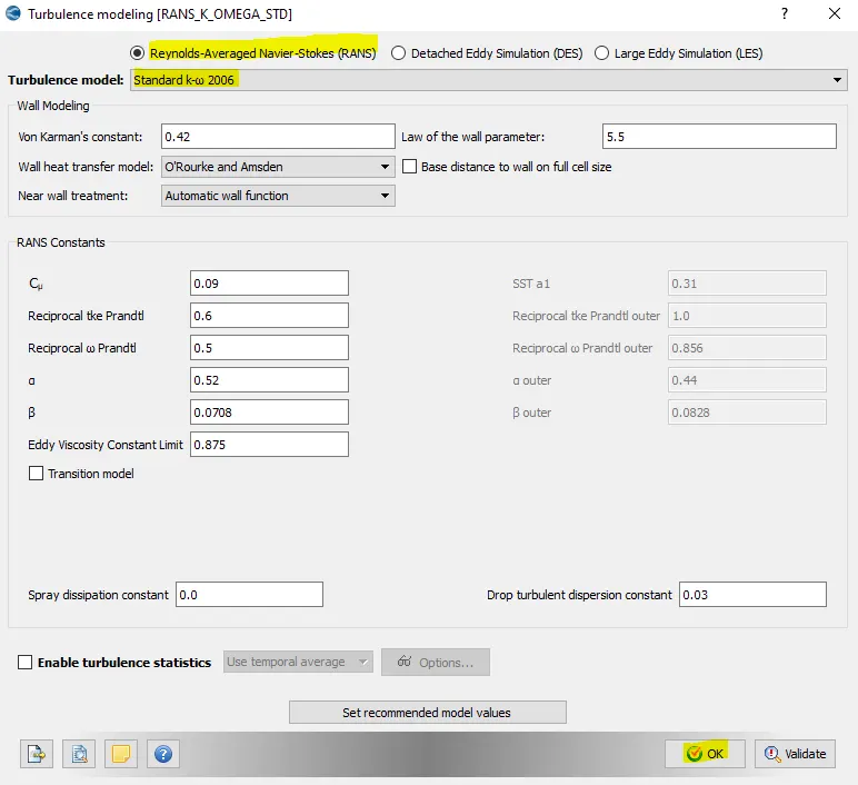
A turbulent model was selected out of so many models. RANS standard K-omega SST model was chosen.

2.7: Grid Control

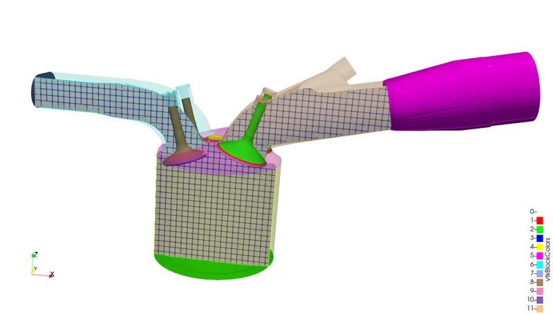
The case study was run using a medium mesh grid size due to less computational resources.

Base mesh sizes are,

S.No.	Dx(m)	Dy(m)	Dz(m)
1	0.004	0.004	0.004

Fixed Embedding

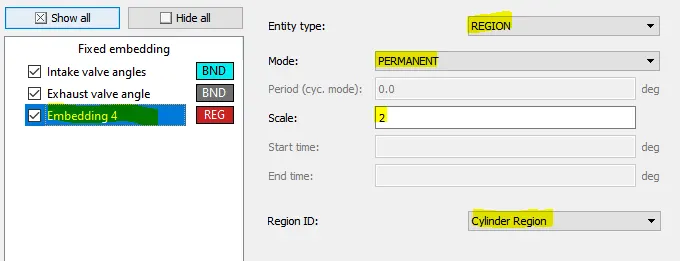
Fixed embedding was done in order to capture more cells near to valve and inside cylinder in order to get more precise data.

Fixed Embedding -1

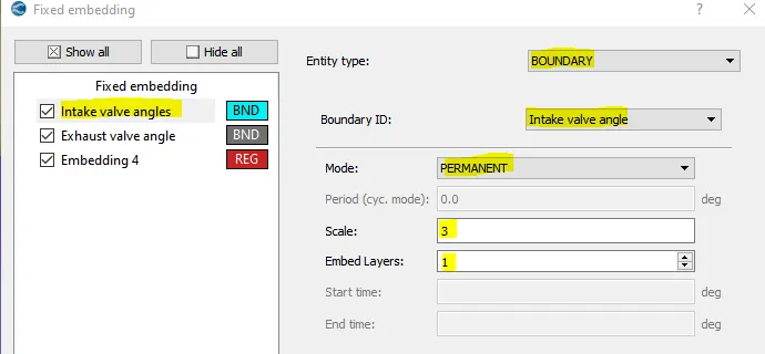
Fixed Embedding -2

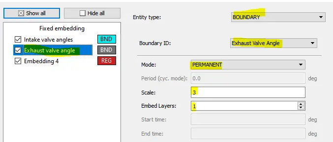
Fixed Embedding -3

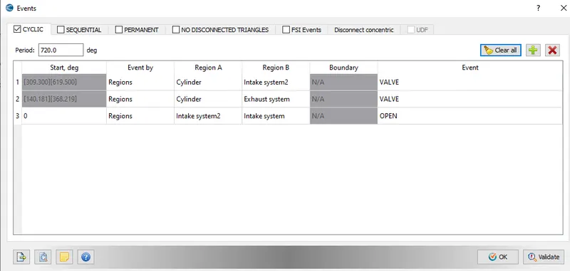
Cyclic event was used in order to establish the pistion mition with respect to crank angle.

4.7 Output/Post-Processing

after regions and initialization are correctly setup.

Also, while setting up the case, make sure, wall output (BOUNDARIES ONLY) is enabled as this will dump wall averaged output data which is very much important for any IC engine simulation

Post-Variable Selection- Existing value

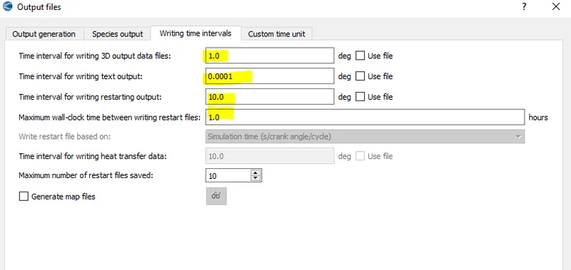
Output Files- Time interval for writing 3D output files-2 deg

The time interval for writing restart files -0.1 deg

The case study was solved using CYGWIN and the post-processing was done in ParaView.

For post converting we used the following command

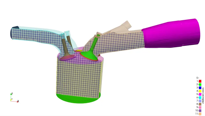
Mesh Geometry

Crank angle =0

Crank angle =80

Crank angle =90

Crank Angle= 120

Crank angle =300

Crank angle =360

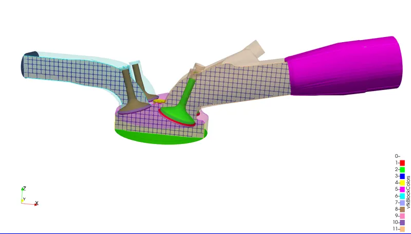
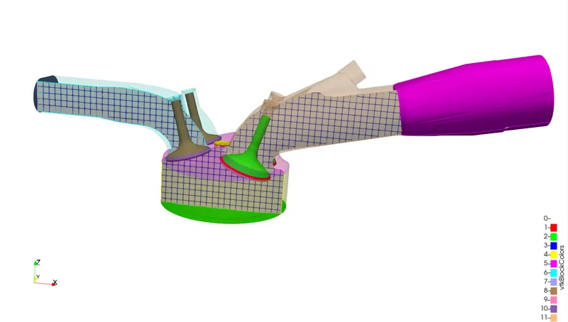
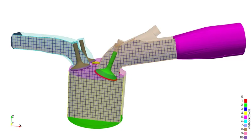
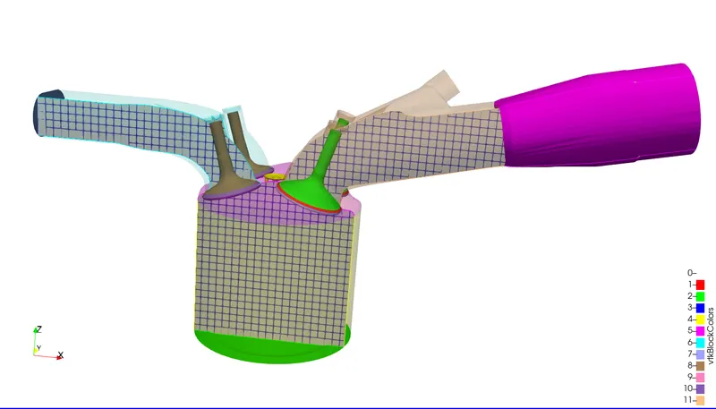
Compression Ratio

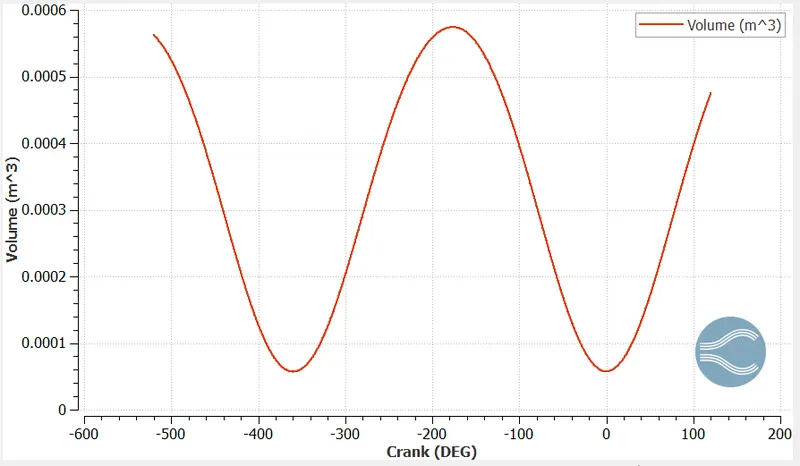
The compression ratio is the ratio between the volume of the cylinder and combustion chamber in an Internal-Combustion Engine at their maximum and minimum values.

In a Piston Engine, the static compression ratio () is the ratio between the volume of the cylinder and combustion chamber when the piston is at the bottom stroke, and the volume of the combustion chamber when the piston is at the top of its strokes.

`CR=(V_d +V_c )/V_c``CR=(V_d +V_c )/V_c=0.000574/(5.72x10^-5)=10.02`

Where:

= displacement volume. This is the volume inside the cylinder displaced by the piston from the beginning of the compression stroke to the end of the stroke.

= clearance volume. This is the volume of the space in the cylinder left at the end of the compression stroke.

Wall Heat Transfer Model

Heat transfer is the transmission of thermal energy through conduction, convection, and radiation. The heat transfer model in FLOW-3D and FLOW-3D CAST solves full conjugate heat transfer equations, accounting for heat transfer within and between fluid, solid and void through conduction, convection and radiation. In order to perform good prediction of engine heat transfer and wall temperature, models are required for accomplish heat transfer from hot gases to engine parts, heat transfer inside each engine part, and also heat transfer to coolant and lubricating oil. CFD simulation study cannot be used to predict the wall temperature.

Combustion Efficiency of Engine

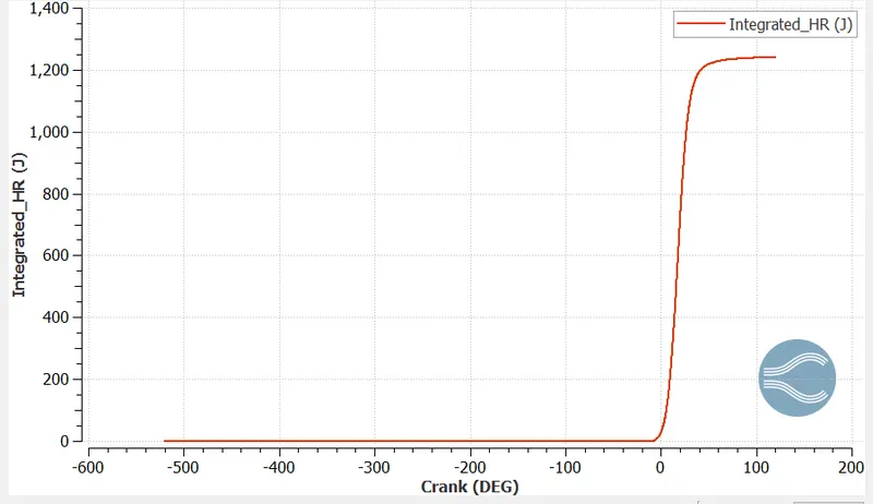
Combustion efficiency is the rate at which an engine converts fuel into energy. Particularly with heavy fuels with high-energy densities — diesel, fuel oil, bunker fuel, etc. — there are technologies available that make it possible to improve combustion efficiency dramatically. Because of the nature of high-energy density fuels, namely that high-energy density fuels are composed of big and long hydrocarbon molecules, heavy fuels can have poor combustion efficiency rates.

Combustion Efficiency is the ratio of total energy released by combustion to the amount of energy contained in the fuel. The Energy containedthe fuel is called lower heating value of calorific value.

Mass of Fuel=`3x10^-5 " kg/cycle"`

LHV - Lower Heating Value of Isooctane=43.44 MJ/kg=`43.44x3x10^-5=1303.2J`

Energy Released fromthe plot=1241.15J

`"Combustion Efficiency"="Energy Released"/"LCV"=1241.15/1303.2=0.952=95.2%`

Power And Torque For the Engine.

Speed=3000rpm=3000/60rps=50 Rev/sec=360*50 degree/sec

Combustion time=240.199 deg

Combustion time in second=240.199/(360*50)=0.0133 s

The net work is given by:-

Work=468.646 N.m

Power=Work/Time

Power=468.646/0.0133=35236.54 N.m/sec

`"Power"=2pi"NT"/60`

`"Torque"=(""Power*"60")/(2piN)`

`"Torque"=468.646/0.0133*60/(2*piN)`

`"Torque"=112.2 W`

Significance of Ca10,Ca50 and Ca90.

Ca10,Ca50 and Ca90 refers to the crank angle at which 10, 50 and 90 percentage of fuel is burnt.

Fom the data obtained using Converge CFD we get following Values:

ca10=6.837

ca50=18.46

ca90=31.7

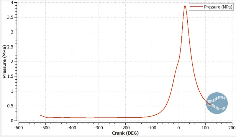
Pressure against Crank Angle

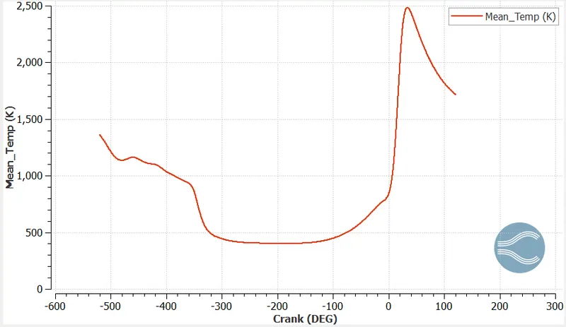
Mean Temperature versus crank angle.

The maxmium mean temperature is oberserved at 22 deg of about 2500K.

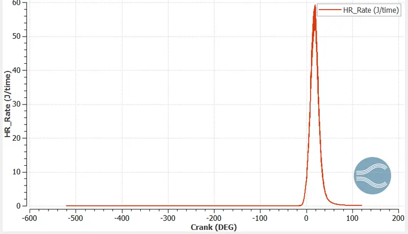
Heat Release Rate Vs Crank Angle

It tells about the amount of heat released per crank angle and per unit time. and it can be noted that the maxmium amount is energy is released at around 22 deg with 59 J/time.

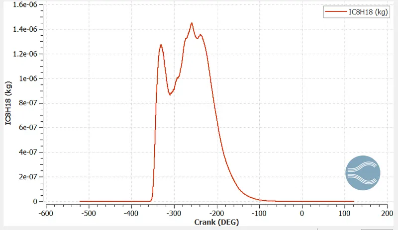
Fuel Spray amount (kg) Versus Crank angle.

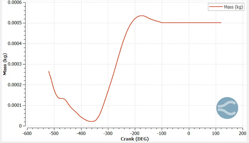
The parcel start to drop after 100 degree its due to vaporization of fuel after some crank angle we dont have fuel left that means no unburnt hydrocarbon.

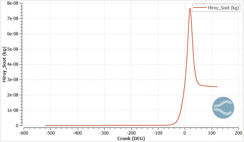
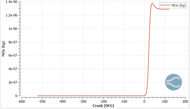
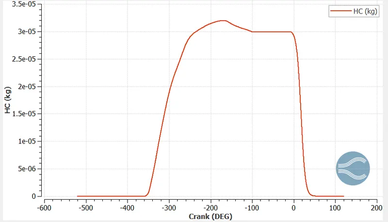
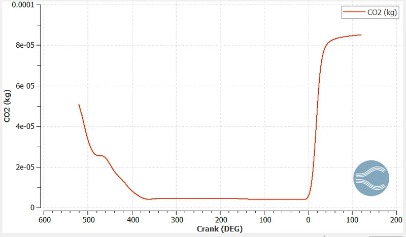
Emissions

Shoot Formation

NOx Emission

Hydro-Carbon

CarbonDiOxide

Animations

The case setup for no hydro can be downloaded from here: https://drive.google.com/file/d/1YdB-Um8AB5ZpQtZxMJVRDfU4Aa9Q-ZzH/view?usp=sharing

Setup for full hydro Port fuel injection setup can be downlaoded from here : https://drive.google.com/drive/folders/145O3KGlw9MLkoA06UOFanmA_-nId6o5w