Second Order Differential Equation to Plot Simple Pendulum using Matlab

Aim

The objective of this project was to just the equation of motion of a simple pendulum with damping and plot the behavior of Simple Pendulum using Matlab.

Introduction

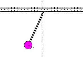
The motion of the simple pendulum can be studied using Ordinary Differential Equation that describes key phenomena and has the ability to solve these equations then you will be able to simulate any of these systems.

This ODE represents the equation of motion of a simple pendulum with damping

`frac{d^2theta}{dt^2}+frac{b}{m}frac{d theta}{dt}+frac{g}{L}sin(theta)=0`

In the above equation,

g = gravity in m/s2,

L = length of the pendulum in m,

m = mass of the ball in kg,

b=damping coefficient.

Converting the Second Order ODE into two first-order ODE

`frac{d^2theta}{dt^2}+frac{b}{m}frac{d theta}{dt}+frac{g}{L}sin(theta)=0`

`theta=thetaunderset{1}{}`

`frac{"d"theta}{dt}=(frac{thetaunderset{1}{}}{dt})=thetaunderset{2}{}`

`(frac{d^2thetaunderset{1}{}}{dt^2})=frac{thetaunderset{2}{}}{dt}`

`frac{"d"thetaunderset{2}{}}{dt^2}+frac{b}{m} thetaunderset{2}{}+frac{g}{L}sin(thetaunderset{1}{})=0`

`frac{"d"thetaunderset{2}{}}{dt^2}=-(frac{b}{m} thetaunderset{2}{}+frac{g}{L}sin(thetaunderset{1}{}))`

Explaination of Code

The equation that was used in this project was 2 order ODE so in order to solve this ODE we have to break this ODE into 2 normal ODE of 1 order. the method is explained above. ODE45 solver in matlab was used for solving the this project. There were many variable, vector and many other codes were used in order to solve this problem.

[t,y]=ode45(@(t,y)simplependulum(t,y),tRange,dis_v);

In the Function calling statement

the function was defined in a function named as simplependulum with tRange as time duration and dis_v as the boundary condition.

The Simple Pendulum was Simulated using Matlab for the motion between 0-20 sec, for angular displacement=0, angular velocity=3 rad/sec2 at time t=0.

Matlab Code

Function name=simplependulum

function dT_dt=simplependulum(t, theta)
   g=9.81
   l=1
   m=1
   b=0.05
    theta1=theta(1)
    theta2=theta(2)
    dT1_dt=theta2;
    dT2_dt=-(b/m)*theta2-(g/l)*sin(theta1)
    dT_dt=[dT1_dt;dT2_dt]
end

Solving Ordinary Differential Equation using ODE45 in Matlab

clc
clear all
close all
l=1;
dis_v=[0;3];
tRange=linspace(0,10,500);

[t,y]=ode45(@(t,y)simplependulum(t,y),tRange,dis_v);

plot(t,y(:,1))
hold on
plot(t,y(:,2))
xlabel('x-Axis')
ylabel('y-Axis')
hold off
title('Angular Displacement V/s Angular Velociy','color','b')

ct=1;
for i=1:length(y(:,1))
    
    x0=0;
    y0=0;
    x1=l*sin(y(i,1));
    y1=-(l*cos(y(i,1)));
    
    figure(2)
    plot([-1,1],[0,0],'linewidth',2)
    hold on
    plot([x0 x1],[y0 y1],'linewidth',2)
    hold off
    hold on 
    plot(x1,y1,"o",'markerfacecolor','g')
    hold off
    
    grid on
    axis([-1.5 1.5 -1.5 0.5])
    M(ct)=getframe(gcf);
    ct=ct+1;
end

figure(3)
movie(M)
videofile=VideoWriter('Spendulum.avi','Uncompressed Avi');
open(videofile)
writeVideo(videofile,M)
close(videofile)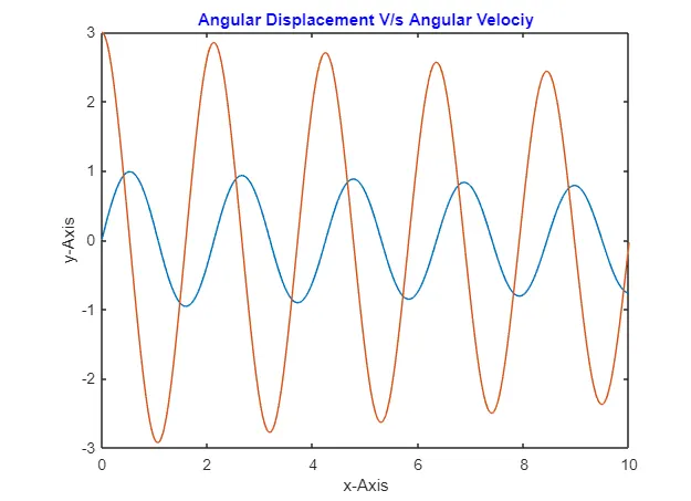

Oscillation Video

Conclusion

The program was executed successfully using Matlab and some damped displacement can be easily seen in the plot means after some time the Pendulum comes to rest.

tRange=linspace(0,300,100);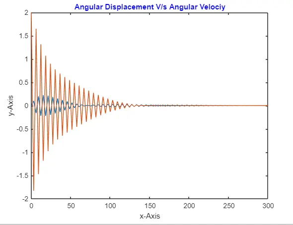

The Code can be downloaded from this link to Drive: Matlab Code for Simple Pendulum