Conjugate Heat Transfer Analysis on a Graphics card Using Ansys Fluent

Aim:

The main objective of this project is to set up steady-state conjugate heat transfer analysis on a Graphics card using Ansys fluent and understand the effect of cooling graphic card by air at 1m/s, 2.5m/s and 5m/s.

The project is further sub-divided into sub-objectives:

1. Running the simulation by varying the velocity from 1m/sec to 5m/sec and post-process the results.
2. Estimation of the maximum temperature and heat transfer coefficient attained by the processor.
3. Prove for result convergence with appropriate images and plots.
4. Identification of potential hotspots on the model.

Introduction:

Conjugate heat transfer is a special case that combines heat transfer in solid and fluid. In the Solid part, conduction dominates whereas fluid part convection dominates. This can be observed in many engineering application like heat exchangers, mufflers cooling ducts, the heat sink is optimized to combine heat transfer by conduction in the heat sink with the convection in the surrounding fluid. Various steps are discussed in this report while making a case set-up for this case study.

Heat transfer in solid is only due to conduction and this is described by Fourier's Law that relates the conductive heat flux(q) is directly proportional to the temperature.

`q=-k nabla T`

whereas time-dependent problem such as transient where temperature field varies with respect to time is given by following partial differential equation:

`rhoC_p (delT)/(delt)=nabla.(knablaT)+Q`

Heat Transfer in a fluid is due to three contribution to the heat equation:

1. The transport of fluid implies energy transport too, which appears in the heat equation as the convective contribution. Depending on the thermal properties of the fluid and on the flow regime, either the convective or the conductive heat transfer can dominate.
2. The viscous effects of the fluid flow produce fluid heating. This term is often neglected, nevertheless, its contribution is noticeable for fast flow in viscous fluids.
3. As soon as a fluid density is temperature-dependent, a pressure work term contributes to the heat equation. This accounts for the well-known effect that, for example, compressing air produces heat.

`rhoc_p (delT)/(delt)+rhoc_pu.nablaT=alpha_pT((delp_a)/(delt)+u.nablap_a)+tau:s+nabla.(knablaT)+Q`

Applications:

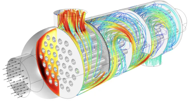
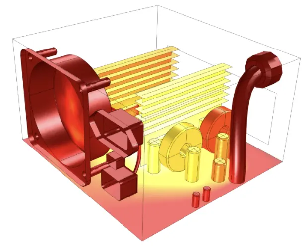
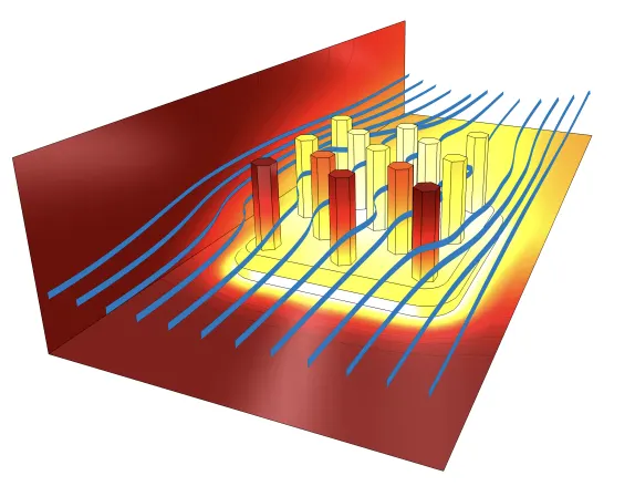
Figure 1 Application of CHT

CHT Modeling Setup

There are several steps to setting up a CHT simulation

1.Define fluid and solid material and their thermophysical properties

2.Configure the fluid and solid regions

3. Assign region to streams.

4. Use appropriate boundary conditions for the boundaries that separated different regions.

5. Select the time control method.

6. Set up post-processing.

1.Geometry Creation:

The Graphic Card assembly Geometry was designed using a separate cad package using Solidworks. Then the geometry was imported to Ansys design modular for future control volume creation as it defines the fluid flow domain important for solid and fluid interaction. The Shared Topology option was enabled to create a common geometry with two different phases for the solid and fluid interface. The fluid flow domain was prepared using the volume preparation option in fluent.

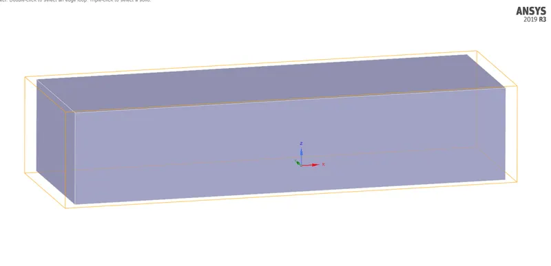
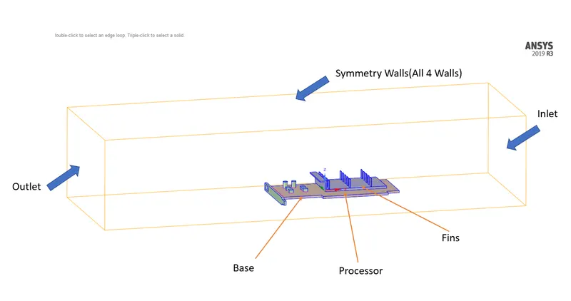
Figure 2. CAD geometry preparation in Ansys Design Modular.

2. Boundary Creation and Meshing

After the control volumes are perfectly created the boundary tags were created in order to assign the different boundary conditions ie. velocity, temperature(if needed), or some other physics. For this geometry, 4 different boundary tags or names were created that were used earlier to assign the boundary condition. The Six names are Inlet, fin, Processor, base, Outlet, and Symmetry walls(all 4 sidewalls).

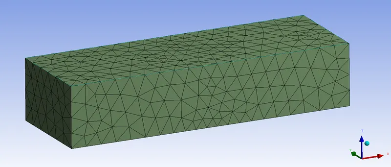
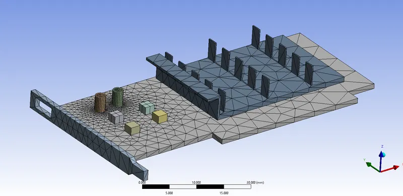
Mesh was generated using yet shape elements, in order to make it more refine the body sizing method for chosen for each named selection.

3. Case Study Setup

For setting up the case study Ansys Fluent was used in order to simulate the case study.

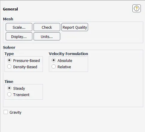
The various parameter was considered while setup this case study. The case study setup dock was used to set up the problem which appears on the left-hand side of the Fluent studio

Solver type: Pressure Based Steady State simulation

S.No.
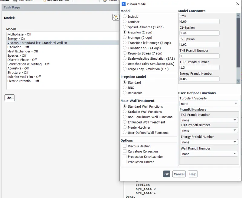
1	Models	Viscous Model-`K-epsilon -"Standard"`	The turbulence model was used as the inlet velocity was too high therefore Reynolds number was in the turbulent category.
2	Material	Air (N2:O2::23%:77%)	Air was used as the fluid inside the Virtual Wind Tunnel
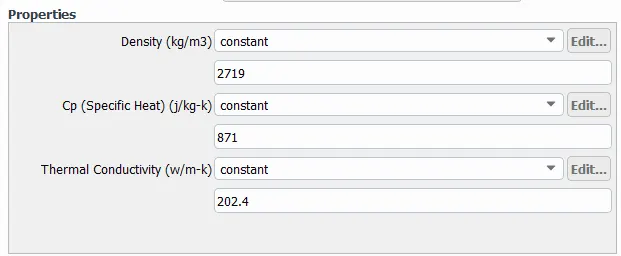
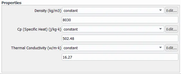
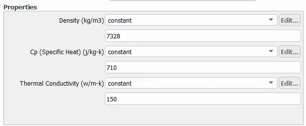
3	Cell Zone Condition	Control Volume Region was set to Air The fin solid part was set to Aluminium The Base solid part was set to Steel The Processor solid part was set to Silicon	The flow inside the Control volume wanted it to be only air.
4	Boundary Conditions	Inlet X is 1m/s, 2.5m/s, and 5m/s
		The outlet was set to 0 Guage Pressure
		The processor was set to heat generation source.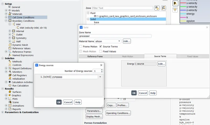
		The remaining walls were set to adiabatic no-slip walls.

From the Literature Review, we know that the normal processor TDP is 1 watt and the volume of the processor from the geometry is 0.008 x 0.008 x 0.001 = 0.00000006 m^3. So, the heat generated by the Processor is calculated to be 1.56 e^7(TDP/Volume). This value is given as the source term for the processor.

Aluminium:

Steel:

Silicon:

4. Solution

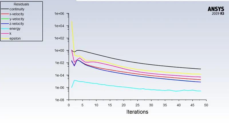
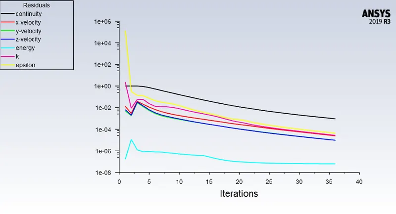
For the Solution Residuals Monitor, the Magnitude was changed to 1e-6 to get more accuracy.

Hybrid Intilizization was used in order to initialize this simulation.

As this was Steady-State Simulation so the Simulation was run for 500 cycles and the results were generated easily.

6.Mesh Independent Study

A Mesh dependency test was performed to select the proper mesh count after which the results stop showing large variation and save a lot of computational time. Three different mesh quality were chosen to study this process.

Mesh Type	Base mesh size(mm)	Number of Nodes	Number of Elements
Coarse Mesh	10.2	15722	87478
Medium Mesh	9 Refinement with Body sizing	41706	236140
Fine Mesh	8 Refinement with Body sizing	123603	721779

The mesh independent test was performed with an inlet velocity of 1m/s.

Case 1: Coarse Mesh

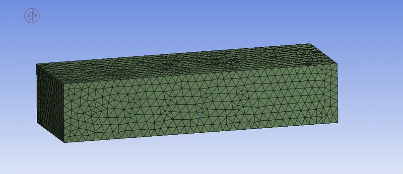
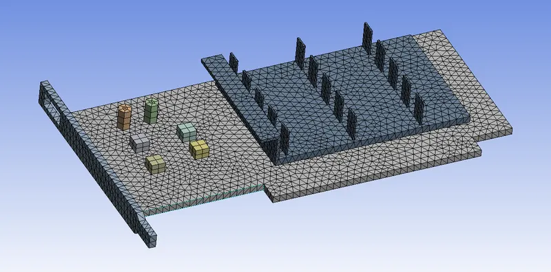
Meshed Geometry

Residual Plot

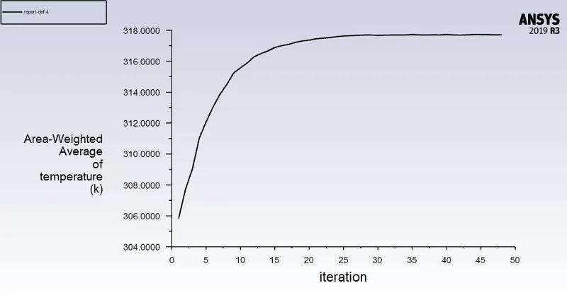
Area Weighted Average Temperature for Fin- Report

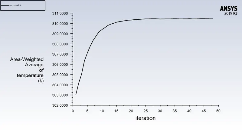
Area Weighted Average Temperature for Base- Report

Post Processing- Result

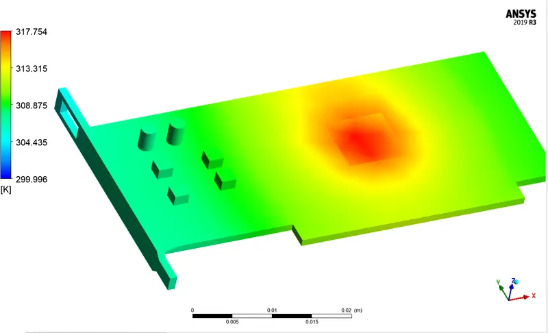
The base of Graphics Card- Temperature-Coarse Mesh

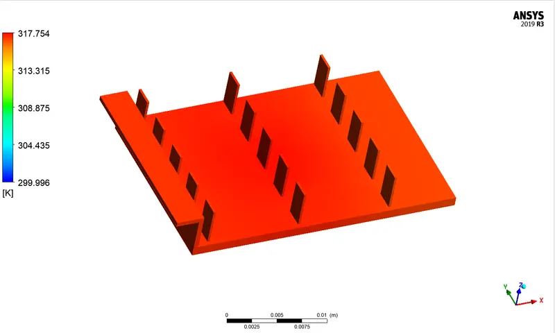
Fins of Graphics Card- Temperature-Coarse Mesh

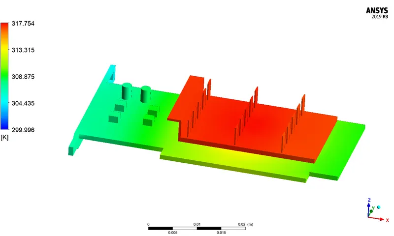
Assembly of Graphics Card- Temperature-Coarse Mesh

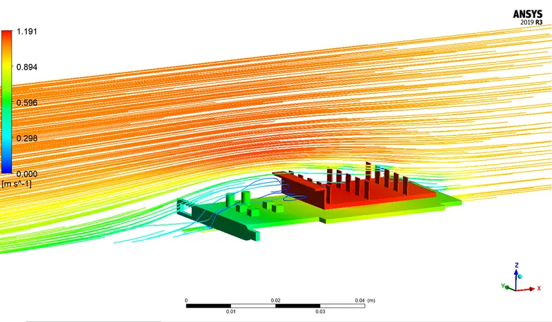
Velocity Stream Lines-Coarse Mesh

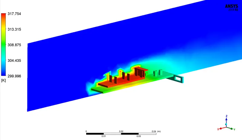
Temperature Contours-Coarse Mesh

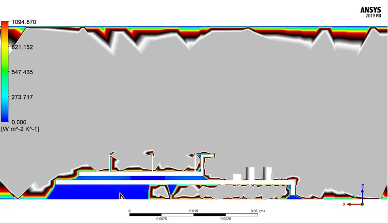
Wall Heat Transfer Coefficient-Coarse Mesh

Case 2: Medium Mesh

Body Sizing

Enclosure Base mesh size is 9mm.

Fin	Element Size=1mm	No Curvature
Base	Element Size=1mm	No Curvature

Residual Plot

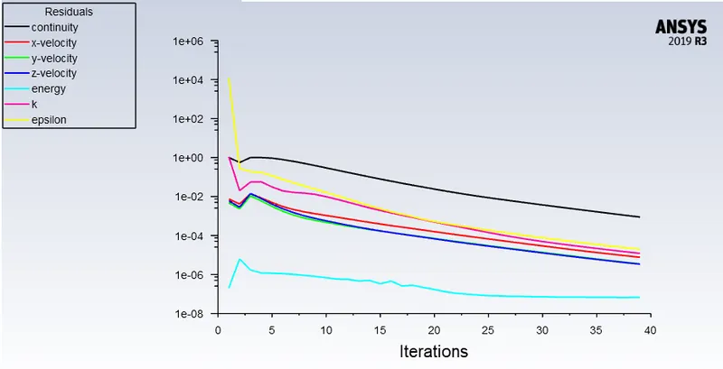
Area Weighted Average Temperature for Fin- Report

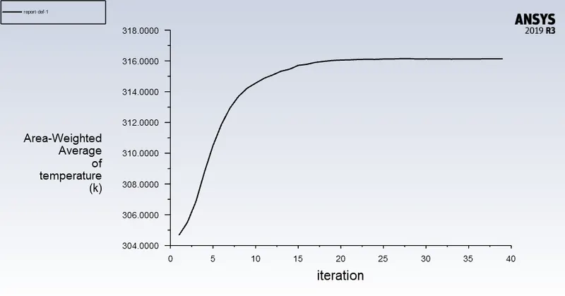
Area Weighted Average Temperature for Base- Report

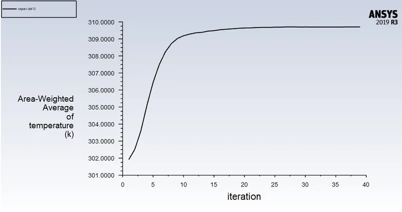
Post Processing- Result

Base of Graphics Card- Temperature-Medium Mesh

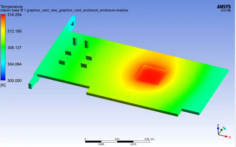
Fins of Graphics Card- Temperature-Medium Mesh

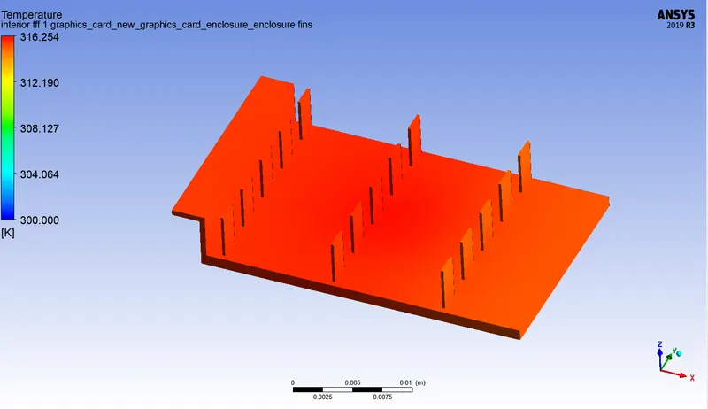
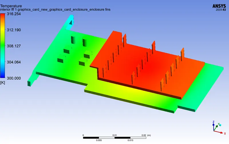
Assembly of Graphics Card- Temperature-Medium Mesh

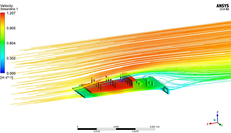
Velocity Stream Lines-Medium Mesh

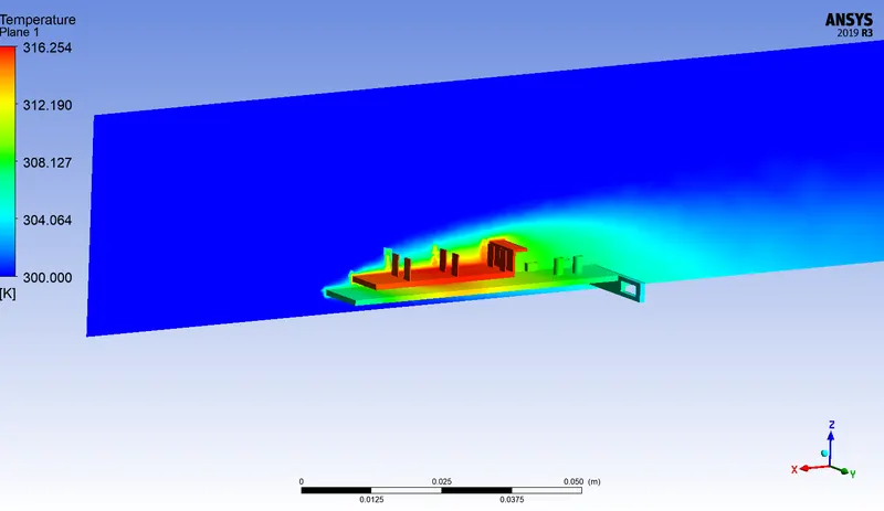
Temperature Contours-Medium Mesh

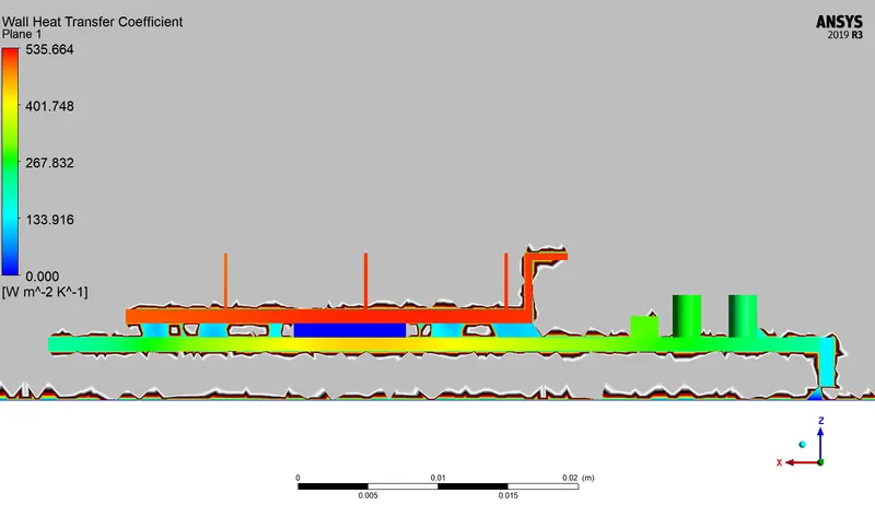
Wall Heat Transfer Coefficient-Medium Mesh

Case 3: Fine Mesh

Body Sizing

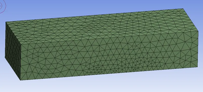
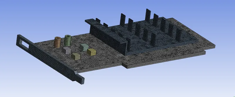
Enclosure Base mesh size is 8mm.

Fin	Element Size=0.4mm	No Curvature
Base	Element Size=0.4mm	No Curvature

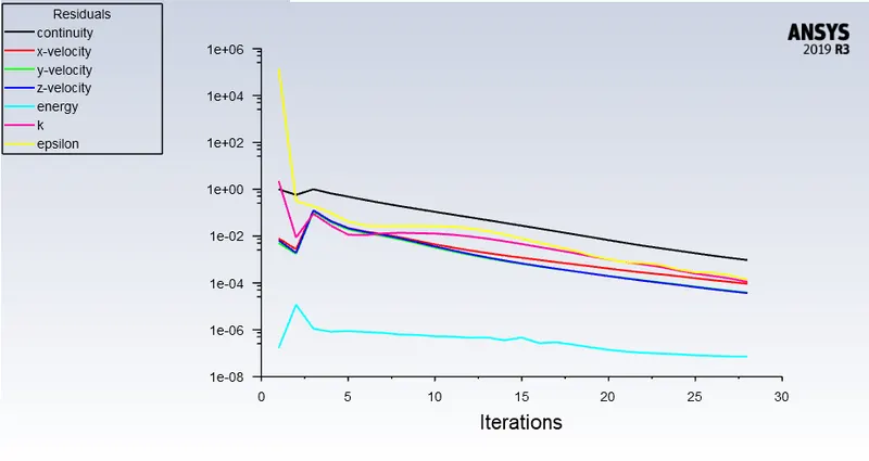
Residual Plot

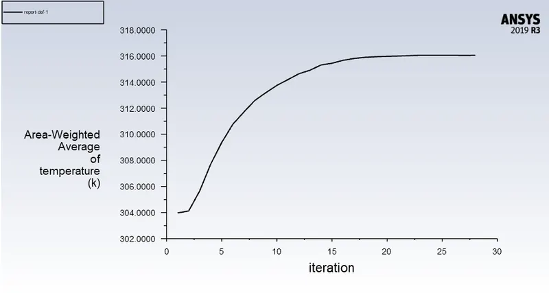
Area Weighted Average Temperature for Fin- Report

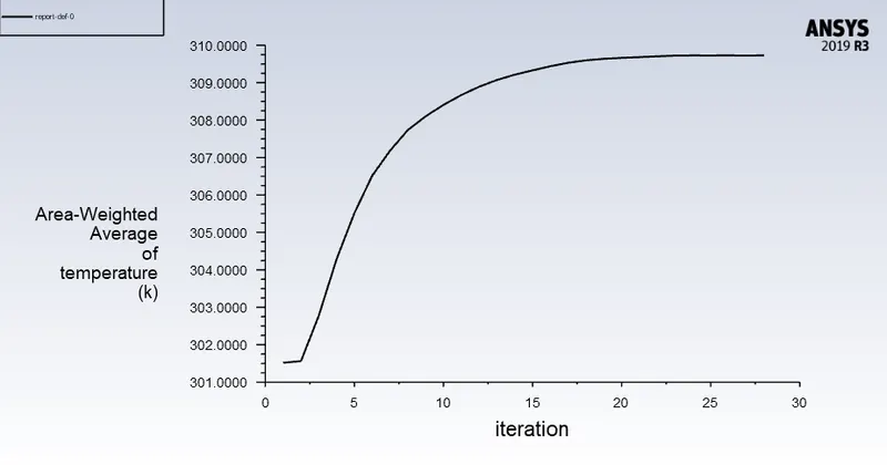
Area Weighted Average Temperature for Base- Report

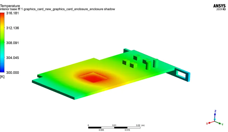
Post Processing- Result

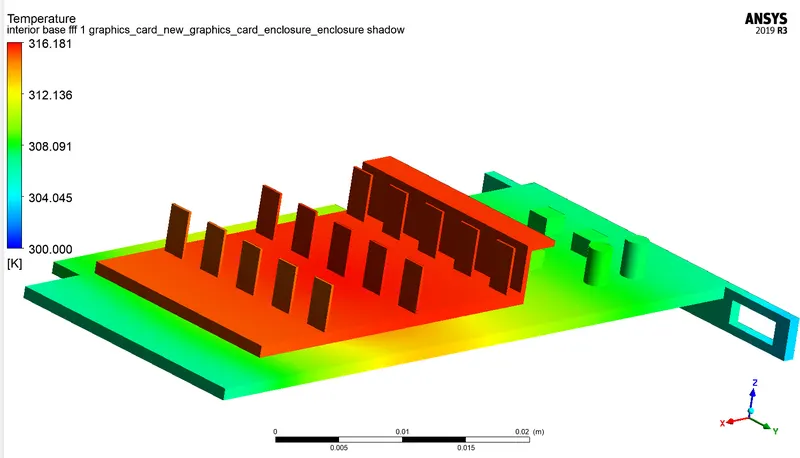
The base of Graphics Card- Temperature-Medium Mesh

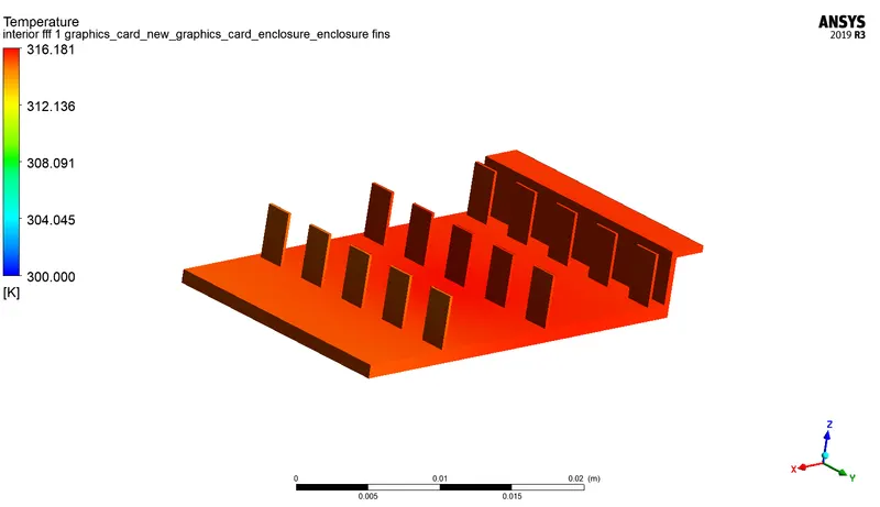
Fins of Graphics Card- Temperature-Medium Mesh

Assembly of Graphics Card- Temperature-Medium Mesh

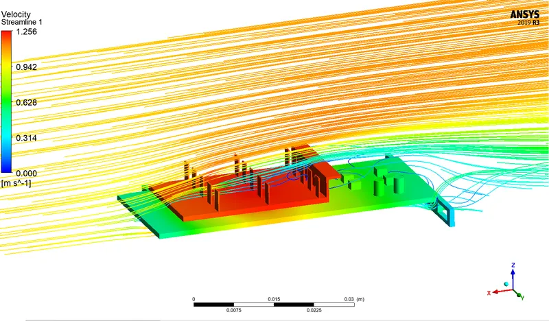
Velocity Stream Lines-Medium Mesh

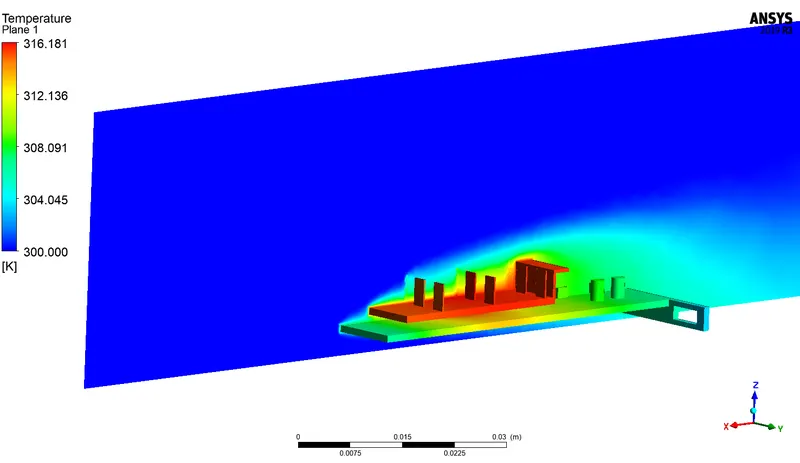
Temperature Contours-Medium Mesh

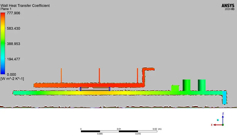
Wall Heat Transfer Coefficient-Medium Mesh

Mesh Independent Study

Three different mesh quality were tested and analyzed. The value of temperature was tracked and a report was generated for this purpose.

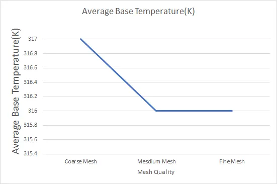
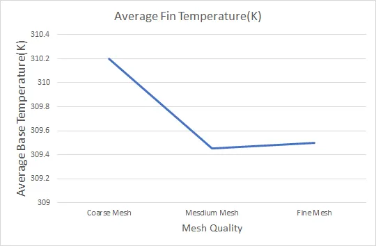
It was observed that the mesh result doesn't show major changes when we further refine the mesh, so the medium quality mesh was chosen for further simulation process

---------------------------------------------------------------------------

Case Study 4 at Velocity 2.5m/s

Residual Plot

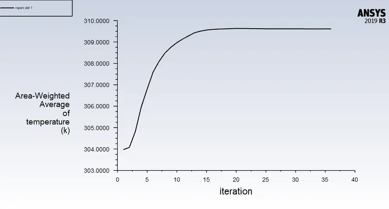
Area Weighted Average Temperature for Fin- Report

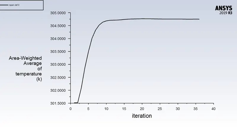
Area Weighted Average Temperature for Base- Report

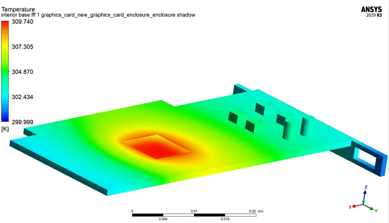
Post Processing- Result

The base of Graphics Card- Temperature-Medium Mesh

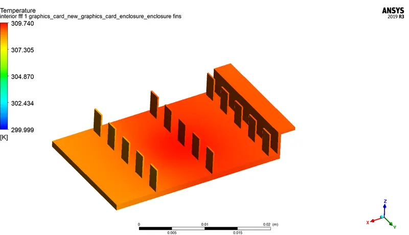
Fins of Graphics Card- Temperature-Medium Mesh

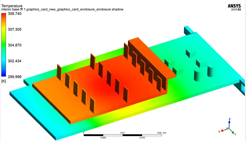
Assembly of Graphics Card- Temperature-Medium Mesh

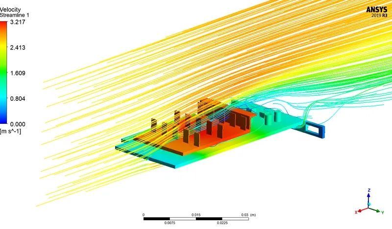
Velocity Stream Lines-Medium Mesh

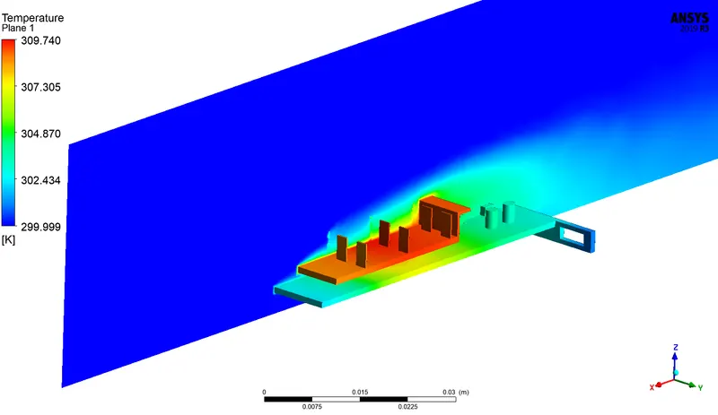
Temperature Contours-Medium Mesh

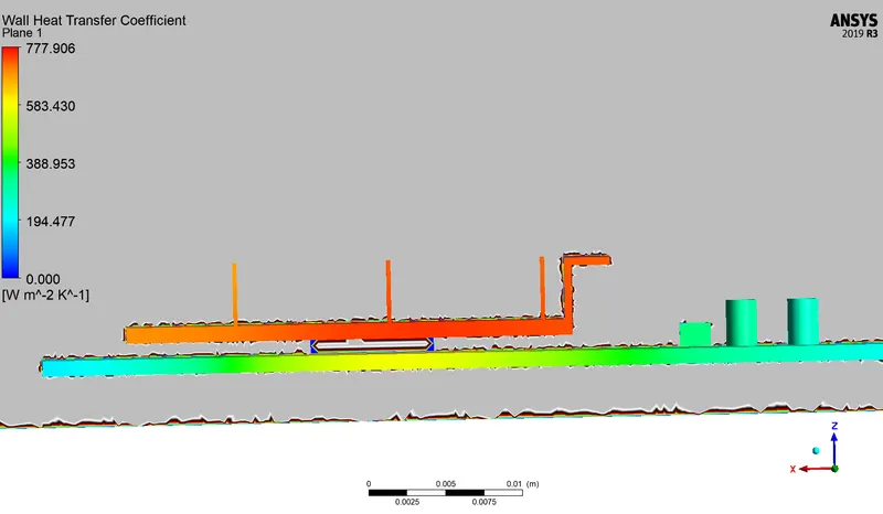
Wall Heat Transfer Coefficient-Medium Mesh

---------------------------------------------------------------------------

Case Study 5 at Velocity 5m/s

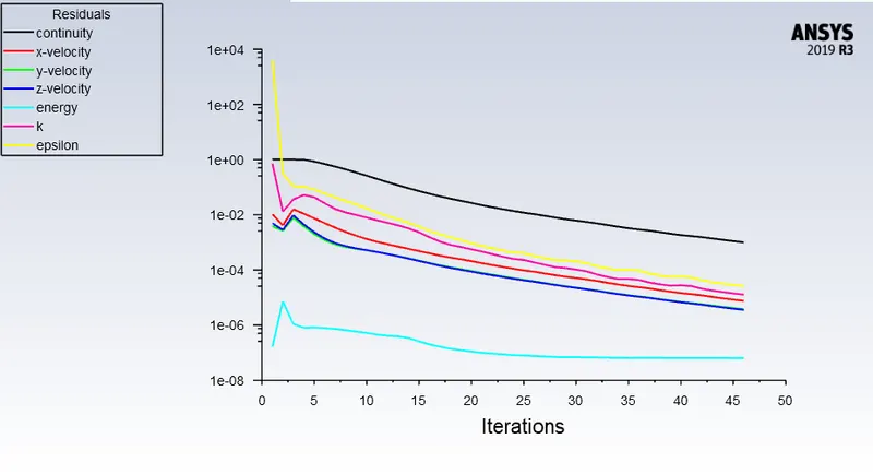
Residual Plot

Area Weighted Average Temperature for Fin- Report

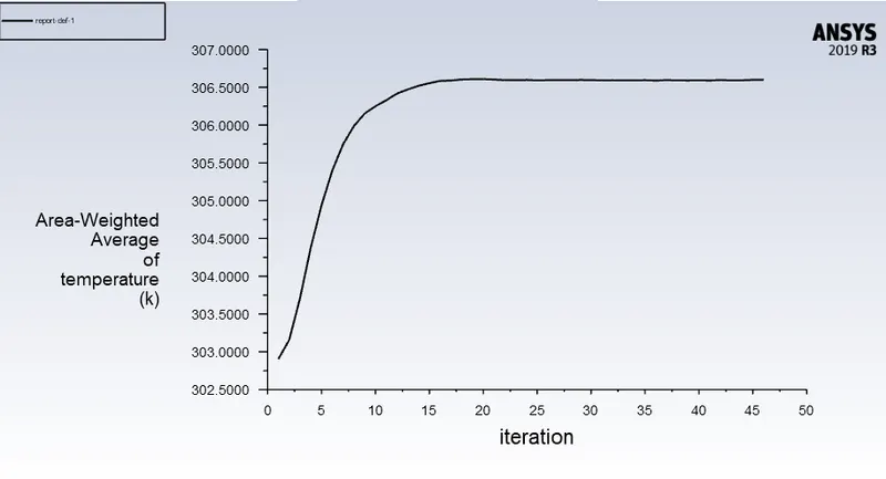
Area Weighted Average Temperature for Base- Report

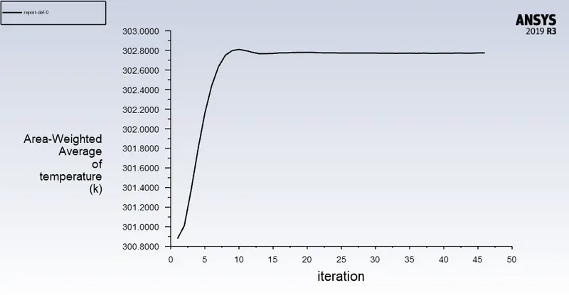
Post Processing- Result

The base of Graphics Card- Temperature-Medium Mesh

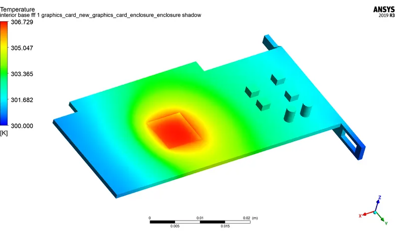
Fins of Graphics Card- Temperature-Medium Mesh

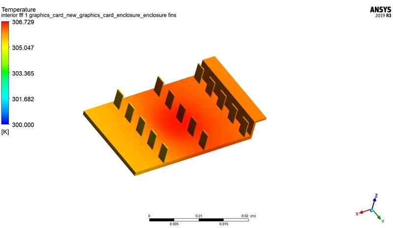
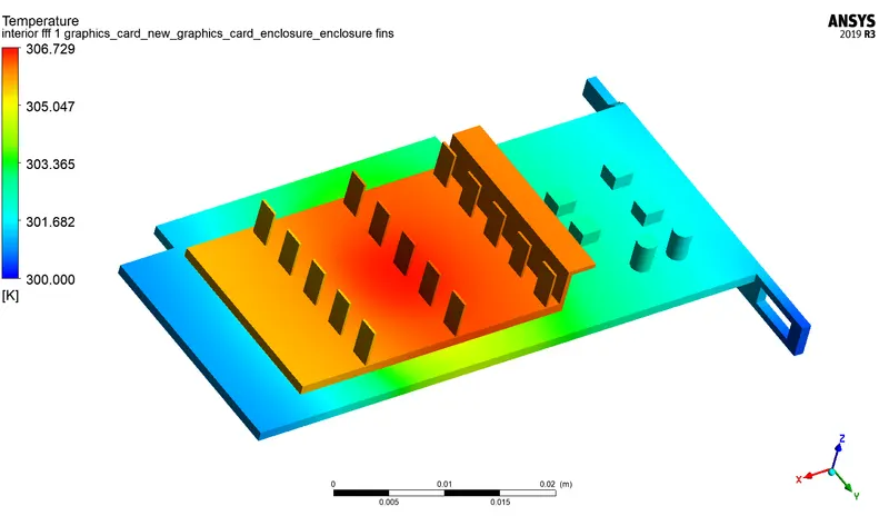
Assembly of Graphics Card- Temperature-Medium Mesh

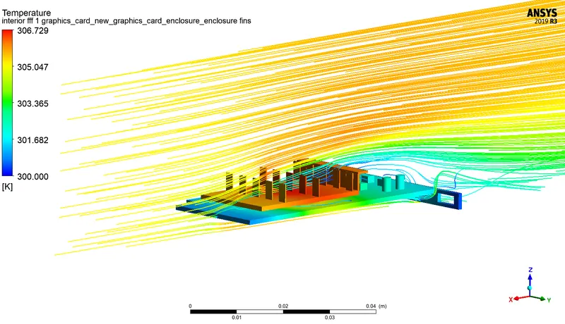
Velocity Stream Lines-Medium Mesh

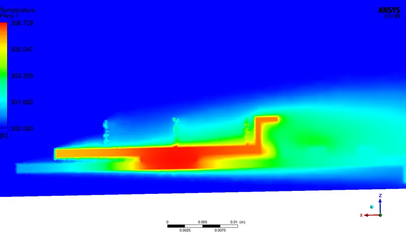
Temperature Contours-Medium Mesh

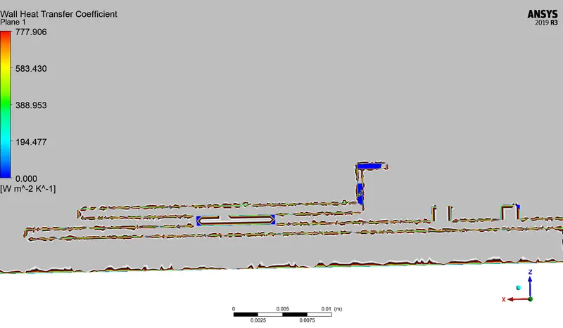
Wall Heat Transfer Coefficient-Medium Mesh

Conclusion

For all the Case study converge result were achieved in steady-state simulation as the results were stable and stopped showing any fluctuations in the values.

The Heat was absorbed by the fin and it was cooled by air which is responsible for heat dissipation in the base and the processor.

Velocity(m/s)	Fin Average Temperature(k)	Base MaximumTemperature(k)	Wall Heat flux(W/m^2 k)
1m/s	309	317	777.77
2.5m/s	309.7	304.55	777.77
5m/s	306	302.7	777.77

as the inlet velocity or the cooling fan speed increases the cooling process also fastens. The major hot spot area can be seen near to processor as that the source of heat generation, it can be observed that the side edges of the base have less temperature and the place where the processor is assembled has a maximum temperature. The fin reduces the temperature of the processor.