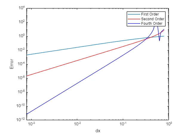
Discretization basics for range of Dx

Aim

The Major objective of this project was to write a Matlab code that can compare the first, second, and fourth-order approximations of the first derivative against the analytical or exact derivative and also Discritize on the basics of Dx

Introduction

The function that will be compute if`F(x)=frac{sin(x)}{x^3}`

The main task was to compute the first Derivative at `x=frac{pi}{3}`

Then compute the derivative both numerically and analytically. Make sure you compute 1st, 2nd, and 4th order derivatives.

Finding an error parameter as the absolute difference in numerical and exact derivative at x = pi/3

First Order Approximation

Function

function out1=firstorder(x,dx)
%analytical Function of Sin(x)/x^3
%f'(x)=(x^3*cos(x)-sin(x)*3*x^2)/x^6;
    analytical_derivative=(x^3*cos(x)-sin(x)*3*x^2)/x^6;
    
    For_diff=((sin(x+dx)/(x+dx)^3)-(sin(x)/x^3))/dx;
    
    out1=abs(For_diff-analytical_derivative);
    
end

Second-Order Approximation

Function

function out2=secondorder(x,dx)
%analytical Function of Sin(x)/x^3
%f'(x)=(x^3*cos(x)-sin(x)*3*x^2)/x^6;
    analytical_derivative=(x^3*cos(x)-sin(x)*3*x^2)/x^6;
    
   CD_1=((sin(x+dx)/(x+dx)^3)-(sin(x-dx)/(x-dx)^3))/(2*dx);
    
 out2=abs(CD_1-analytical_derivative)
    
end

Fourth-Order Approximation

Function

function out4=fourthorder(x,dx)
%analytical Function of Sin(x)/x^3
%f'(x)=(x^3*cos(x)-sin(x)*3*x^2)/x^6;
    analytical_derivative=(x^3*cos(x)-sin(x)*3*x^2)/x^6;
    
    CD_4=(((sin(x-2*dx)/(x-2*dx)^3))-8*((sin(x-dx)/(x-dx)^3))+8*((sin(x+dx)/(x+dx)^3))-((sin(x+2*dx)/(x+2*dx)^3)))/(12*dx)
    
    out4=abs(analytical_derivative-CD_4)
    
end

Matlab Code For Computation and Discretization basics for a range of dx in order to what happens if we refine the mesh.

clear all
close all
clc

x=pi/3;
dx=linspace(pi/4,pi/4000,20);

for i=1:length(dx)
    %First order Approxmiation
    First_order(i)=firstorder(x,dx(i));
    %Second Order Approxmiation
    Second_Order(i)=secondorder(x,dx(i));
    %Fourth Order Approxmiation
    Fourth_Order(i)=fourthorder(x,dx(i));
end

loglog(dx,First_order)
hold on
loglog(dx,Second_Order,'r')
loglog(dx,Fourth_Order,'b')
hold off
legend('First Order','Second Order', 'Fourth Order')
xlabel('dx')
ylabel('Error')

Explanation

For the creation of Dx, the linspace command was used in order to create the 20 values that are equally distributed from `{frac{pi}{4}tofrac{pi}{4000}}`

dx=linspace(pi/4,pi/4000,20);

For Loop was used in order to store and compute the value at different values of Dx

for i=1:length(dx)
    %First order Approxmiation
    First_order(i)=firstorder(x,dx(i));
    %Second Order Approxmiation
    Second_Order(i)=secondorder(x,dx(i));
    %Fourth Order Approxmiation
    Fourth_Order(i)=fourthorder(x,dx(i));
end

At last, the Plot was plotted using the Log Scale

loglog(dx,First_order)
hold on
loglog(dx,Second_Order,'r')
loglog(dx,Fourth_Order,'b')
hold off
legend('First Order','Second Order', 'Fourth Order')
xlabel('dx')
ylabel('Error')

Plot