CFD Simulation of Dassault Rafale using Converge CFD
Aim:
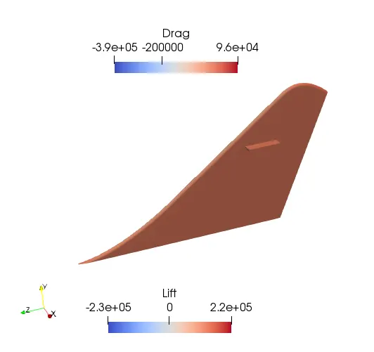
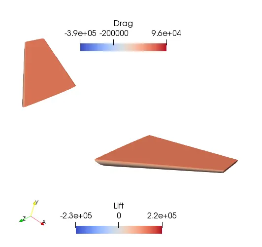
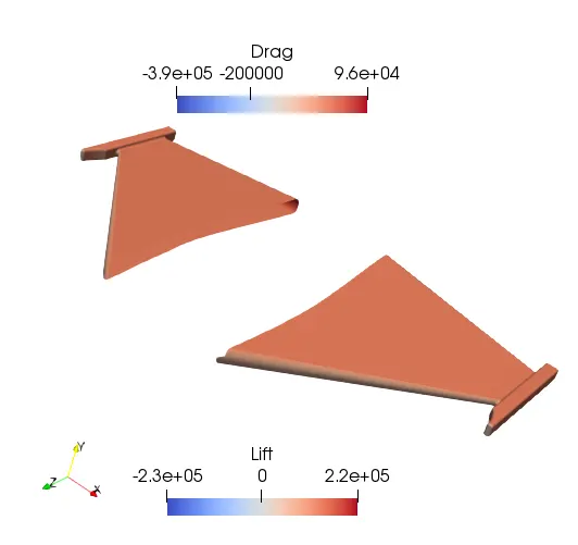
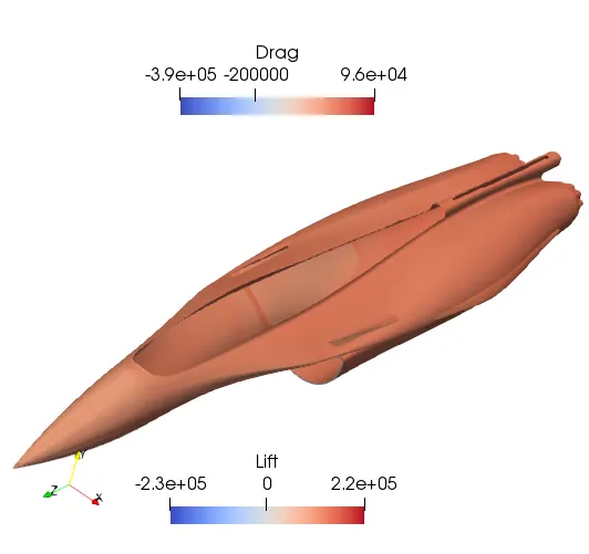
The major objective of this project was to Setup flow around Dassault Rafale using Converge CFD and Estimate the Drag and Lift force on different major components.
Introduction:
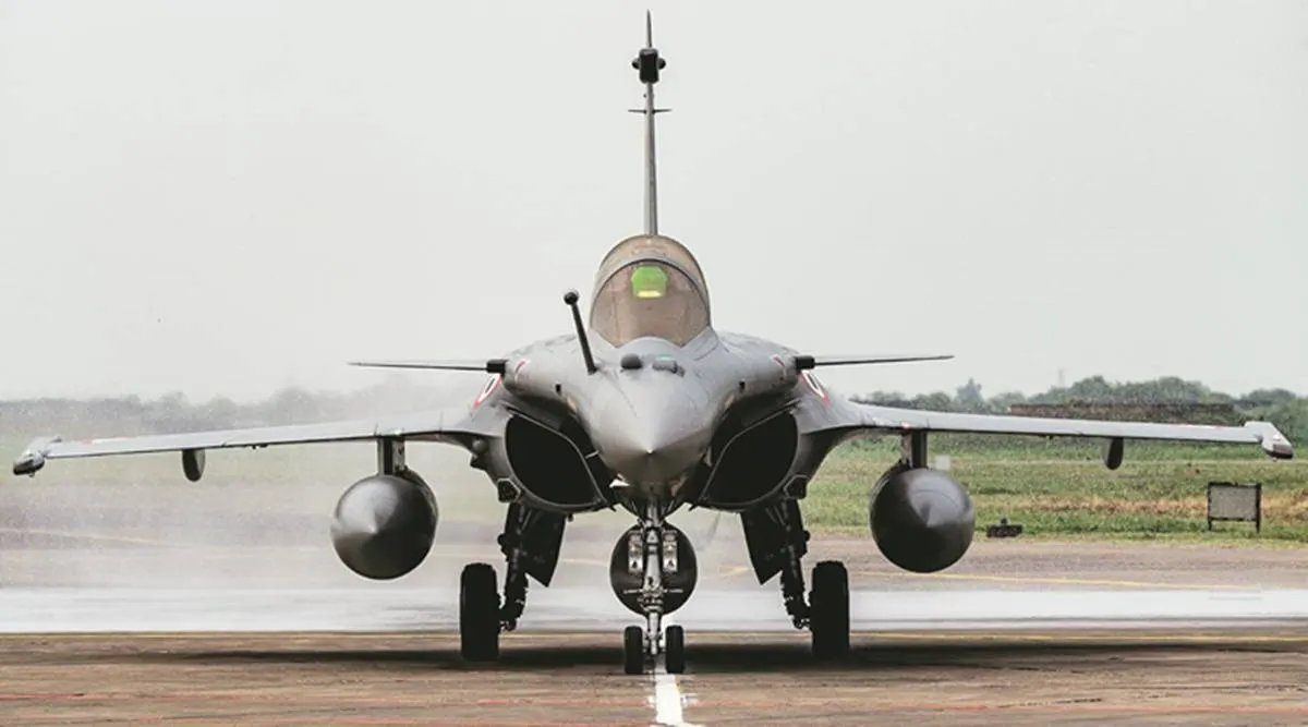
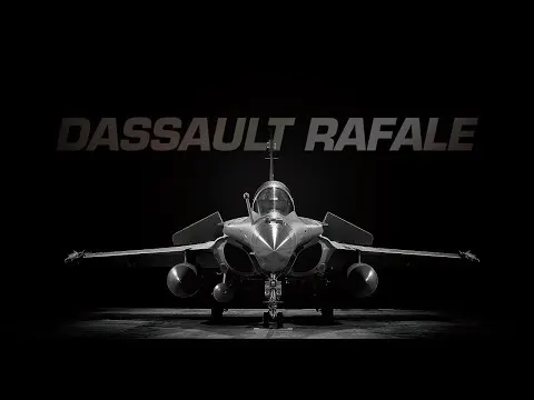
The Rafale is a twin-jet fighter aircraft able to operate from both an aircraft carrier and a shore base. The fully versatile Rafale is able to carry out all combat aviation missions: air superiority and air defense, close air support, in-depth strikes, reconnaissance, anti-ship strikes, and nuclear deterrence. The Rafale entered service with the French Navy in 2004 and with the French Air Force in 2006. With more than 30,000 flight hours in operations, it has proven its worth in combat in Afghanistan, Libya, Mali, Iraq, and Syria. The Rafale was ordered by Egypt, Qatar, and India.
The project mainly focuses on the following things:-
1. Importing the(.Stl) file on Converge Studio then cleaning up the geometry removing the intersection, patching the new open edge, deleting the unwanted edge, and Fixing the normal orientation of the geometry.
2. Creating Virtual Wind Tunnel using proper Dimension.
3. Case Setup using Converge Studio using proper Solver and Boundary Conditions.
4. Solving the Case Study Files using Cygwin.
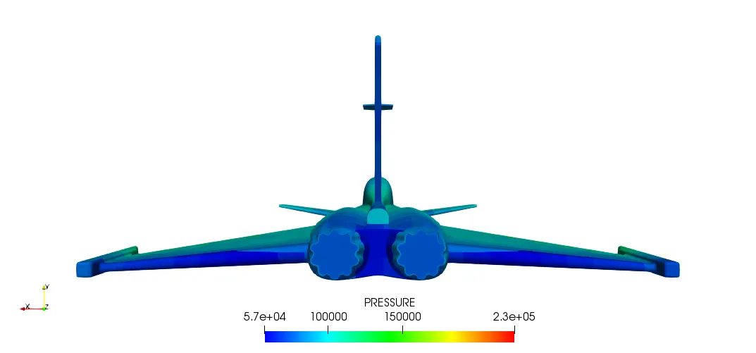
5. Post-Processing the result Using ParaView generating Velocity, Pressure, and y+ contours.
6. Generating the plots and comparing the result for Drag and Lift force using Ms. Excell.
--------------------------------------------------------------------------------
1. Importing the Geometry for Geometry Clean Up using Converge Studio
Firstly the Geometry(.stl) was imported in Converge Studio. The diagnostic tool was used to find the open edge, Intersection edges, and other errors like orientation error. Many features were used to repair the geometry like 1. Deleting the edge, node, face. 2. Patching the edge using the patch tool. 3. Stitching the two misalign edges.
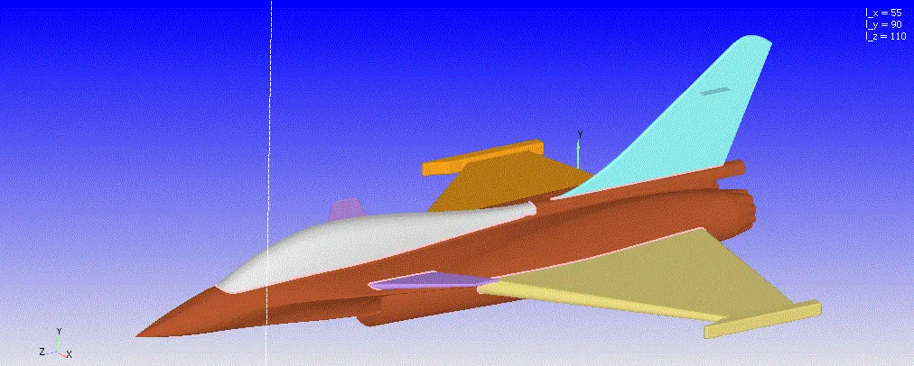
The Rafale geometry that was provided had Many total open edge errors. so geometry cleaning plays an important role in setting up a simulation of a Rafale. There were many features that were used to clean the geometry. First, the geometry was checked using the Diagnostic tool to check what kind of error is present then our main target was to repair an open edge without forming an intersection.
First, the surface(Triangle) was deleted shown in green color then the extra edges were removed to make a perfect open loop that can be patch letter. For patching those new open edge the edges were checked and patch repair option was used to patch the open edge method. Then the geometry was checked again to find any error.
The normal orientation was fixed using automatic option present in Transform>Normal> Automatic fix all the normals.
Case Study Set-Up
1.Geometry Creation
First of all, the Rafale geometry was imported using converge CFD software. The geometry was separately prepared using different CAD package ie Solidworks, then .stl file was imported to Converge Studio to set up the case study. Then the geometry clean up was performed in order to check for errors.
The Geometry was scaled using proper scale because the geometry was prepared using Inch so for that the geometry was converted in Metre using Scale feature.
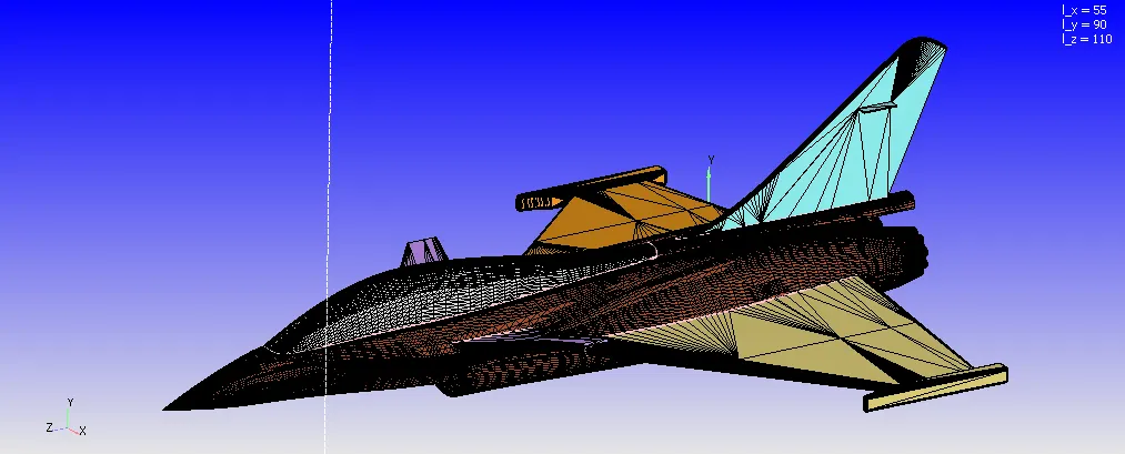
After the geometry was cleaned than the Virtual wind tunnel was created.
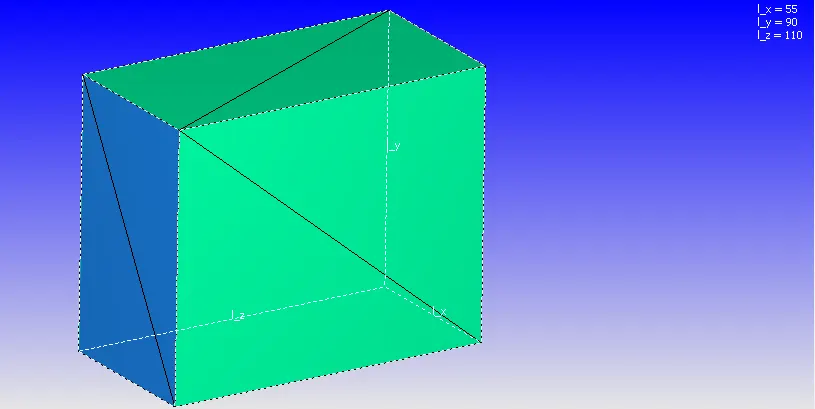
The Virtual Wind Tunnel Dimension for this Case Study is :
| Dx(m) | Dy(m) | Dz(m) |
| 55 | 90 | 110 |
To create the geometry, the geometry was uploaded from the different CAD software package. All the normal vector were pointing out for this geometry, so we wanted it to point inside and normal to each surface. Normals point the direction of the fluid region generally. The command "Transform" was used to make the normal inside pointing the direction of the fluid region.
2.Boundary Creation
After creating the Geometry along with Wind Tunnel Geometry, The Boundry tag was created along with different boundary id and coloring. A total of 9 different boundaries tag was created for multiple different split triangles of the geometry with each face split into multiple triangles. To create the boundaries naming, the "Boundary" command in the "Geometry" dock was used, and then the faces were appointed to appropriate tags along with id.
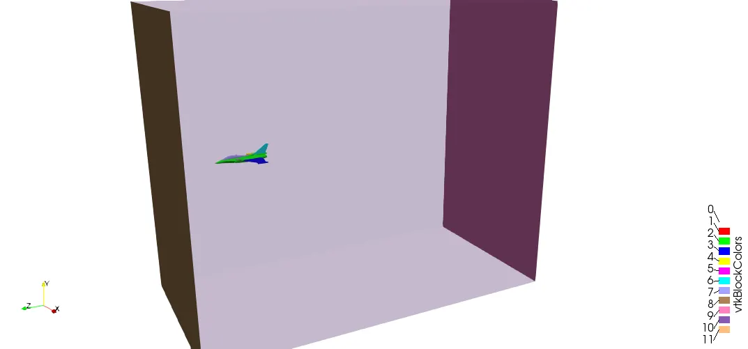
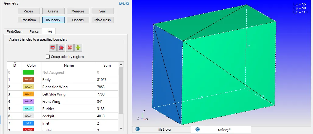
First, the Geometry was split into many parts using Boundary Fencing Method using those parts the Boundary tag was created.
Then the Inlet, Outlet, and Symmetry walls were created.
3.Case-Study Setup
The various parameter was considered while setup this case study. The case study setup dock was used to set up the problem which appears on the right-hand side of the converge studio.
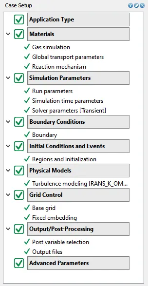
3.1 Application Type:
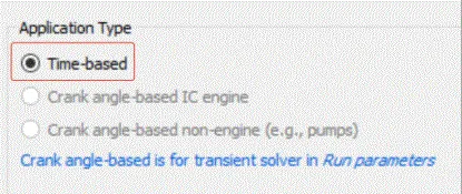
In order to run a steady-state simulation, firstly, under the Application type in the setup tree, a "Time-based" simulation must be selected.
3.2 Materials:
Under the material tab "Gas simulation" was selected and "Air" as a predefined mixture.
Gas: Air
Global Transport Parameters: Fixed value
by default, the following value is considered.
Prandtl Number : 0.9
Schmidt Number : 0.78
Species: Oxygen-O2 & Nitrogen-N2
3.3 Simulation Parameters
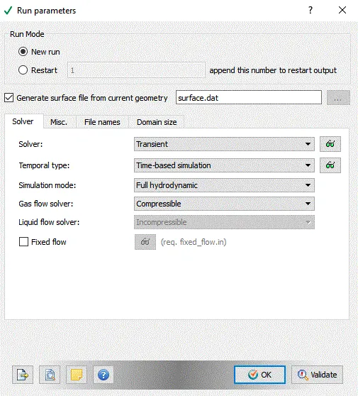
The Transient solver was selected for running this case study along with a "Density-based" solver.
 .
.
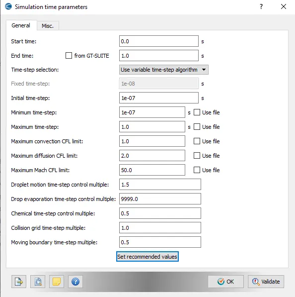
Calculation
Horizontal length=110m
Average Velocity for Case 1=385m/s
Speed=Distance/time
therefore, Time=0.2857 sec
we are simulating roughly 4 times of flow through time that is 1s
The Following Simulation parameters were selected for running this simulation.
3.4: Boundary Conditions
In this tab, The volumetric region and physics for each boundary were defined.
| Boundary_Name | Boundary_Type | Paramter_Defined | Boundary ID |
| 1. Body | Wall | Law of Wall | 1 |
| 2. Rear Side Wings | Wall | law of Wall | 2 |
| 3. Left Side Wings | Wall | law of Wall | 3 |
| 4. Front Wing | Wall |
law of Wall |
4 |
| 5. Rudder | Wall | law of Wall | 5 |
| 6. Cockpit | Wall | law of Wall | 6 |
| 7. Inlet | Inflow |
385 m/s in -Z-axis Case2 (Dirichlet Boundary Condition) The pressure being at NE (Neuman Boundary condition) |
7 |
| 8. Symm Wall | Symmetry | law of Wall | 9 |
| 9. Outlet | Outflow |
101325.0 Pa at 300 k (Dirichlet Boundary Condition) |
8 |
3.5: Initial Conditions and Events
Volumetric Region was created in order to assign this to all the boundary tag.
Species:- O2 (0.23) & N2 (0.77)
Pressure :101325Pa
Temperature:300K
The velocity of 385m/s in -X-axis
3.6: Physical Models
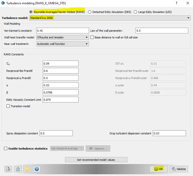
A turbulent model was selected out of so many models. RANS standard K-omega SST model was chosen.
3.7: Grid Control
The case study was run using a Coarse mesh grid size due to less computational resources.
Base mesh sizes are,
| S.No. | Dx(m) | Dy(m) | Dz(m) |
| 1 | 2.0 | 2.0 | 2.0 |
Fixed Embedding
Fixed embedding was done in order to capture more cells near to throttle in order to get more precise data.
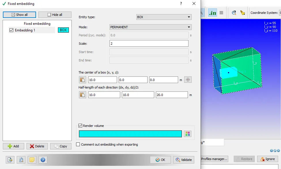
The wind tunnel has a box embedded inside with more fine computational cells in order to capture more data more precisely.
3.7 Output/Post-Processing
In regions and initialization, the value of velocity should be the same as that of Inlet velocity.
Also, while setting up the case, make sure, wall output (BOUNDARIES ONLY) is enabled as this will dump wall averaged output data which is very much important for any external aerodynamic simulations.
Post-Variable Selection- Existing value
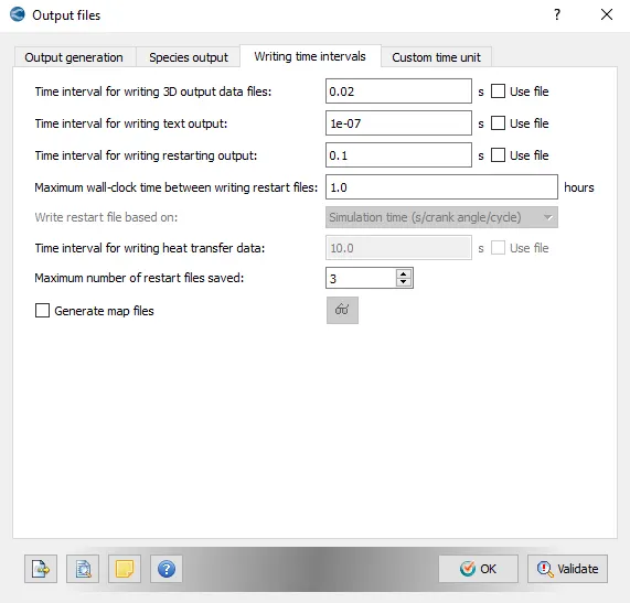
Output Files- Time interval for writing 3D output files-0.018 s
The time interval for writing restart files -0.1s
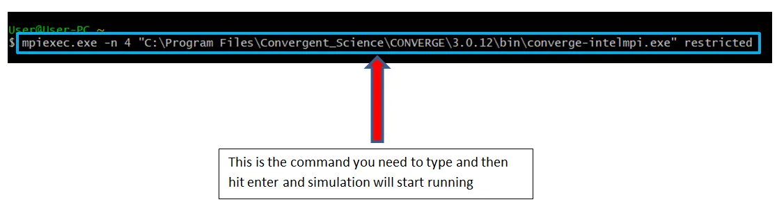
The case study was solved using CYGWIN and the post-processing was done in ParaView.
Simulation Results
Mesh Model
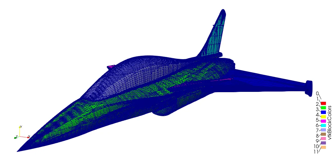
Simulation Result
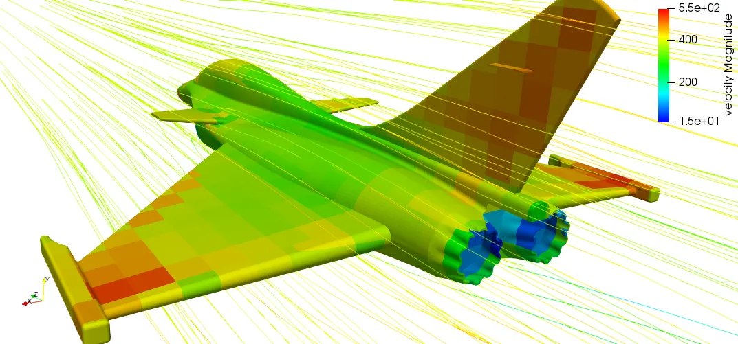
Velocity Contour
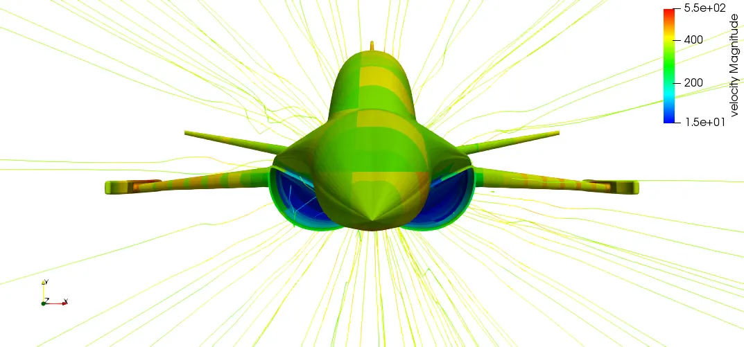
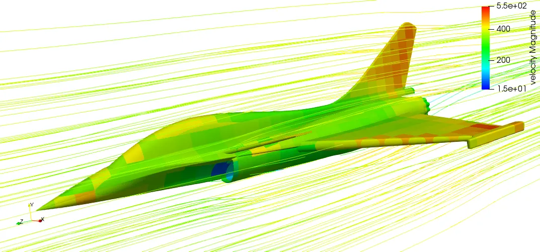
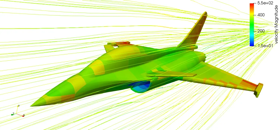
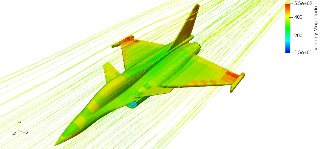
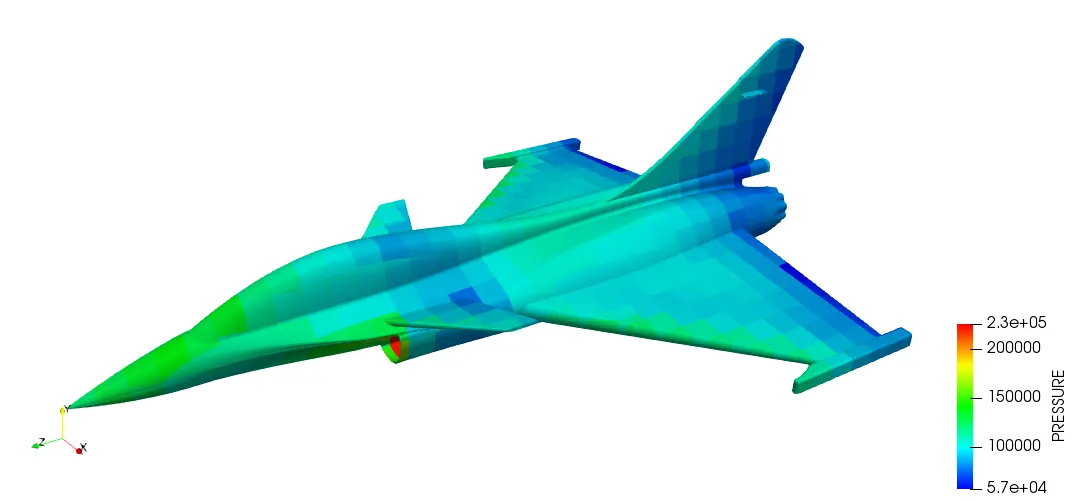
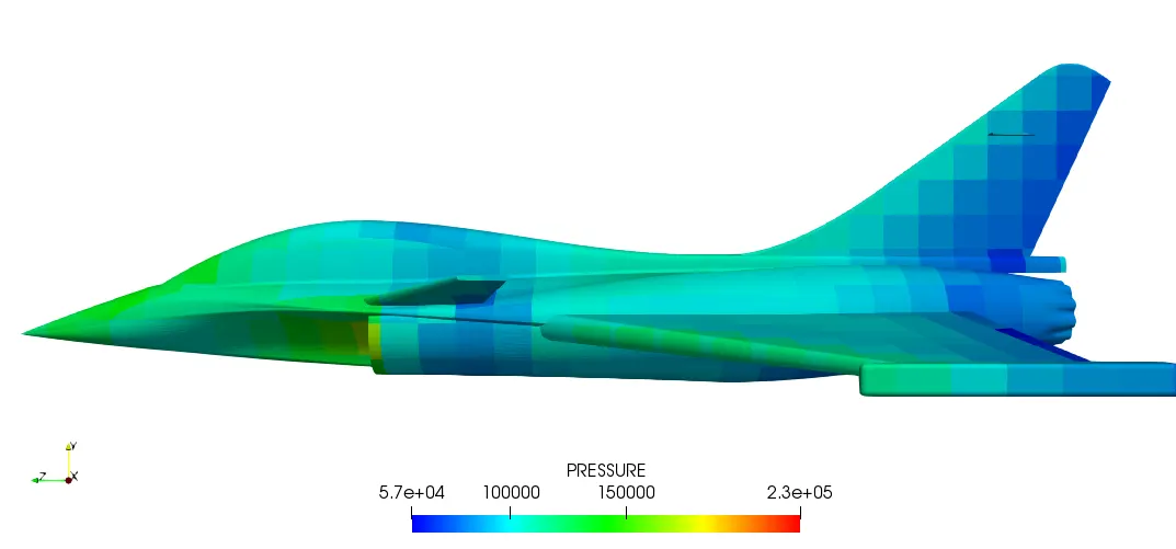
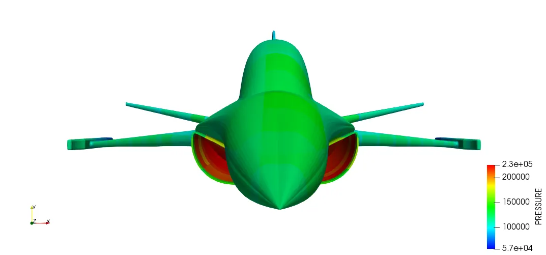
Pressure Contour
Y Plus
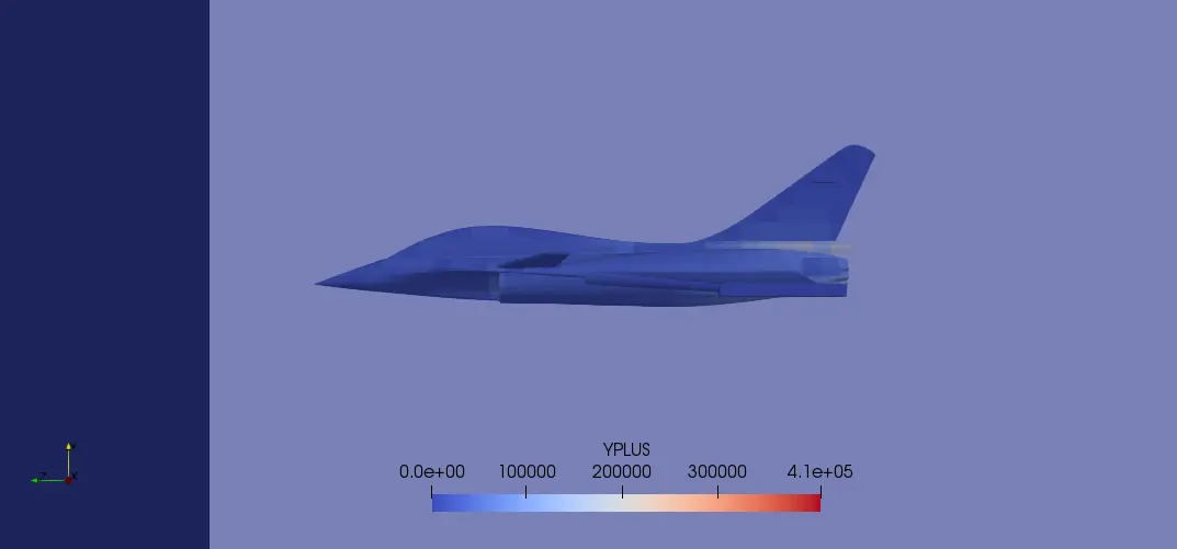
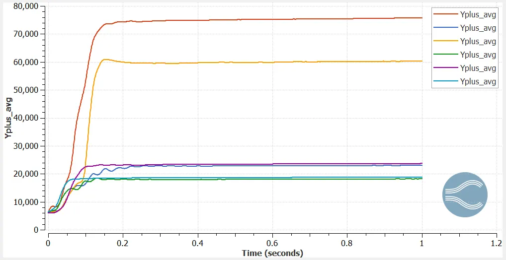
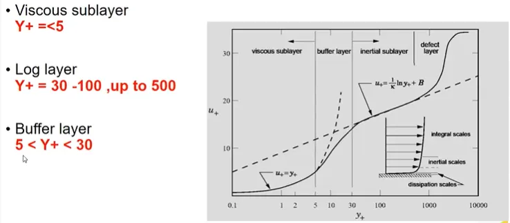
Turbulence is the state of chaotic and unstable fluid flow, just opposite of Laminar flow. Y plus(Y+) is the non-dimensional distance of the first cell from the wall.
Let's takes an example of a flat plate under zero pressure gradient and front left side the uniform velocity is coming to the plate. Firstly, it will be laminar flow, then after some disturbance, the region will be called as Transition Region, when the disturbance is growing too much the flow will change in Turbulent Flow. The boundary layer in the turbulent region will be called a turbulent boundary layer whereas in laminar it will be called the laminar boundary layer.
Reynold's Number `Re` is the ratio of Inertial force to the Viscous Force.
Viscous Sub Layer: Viscous stress term dominates
Buffer Layer: Transitional region
Log law Region: Reynolds shear stress term dominates
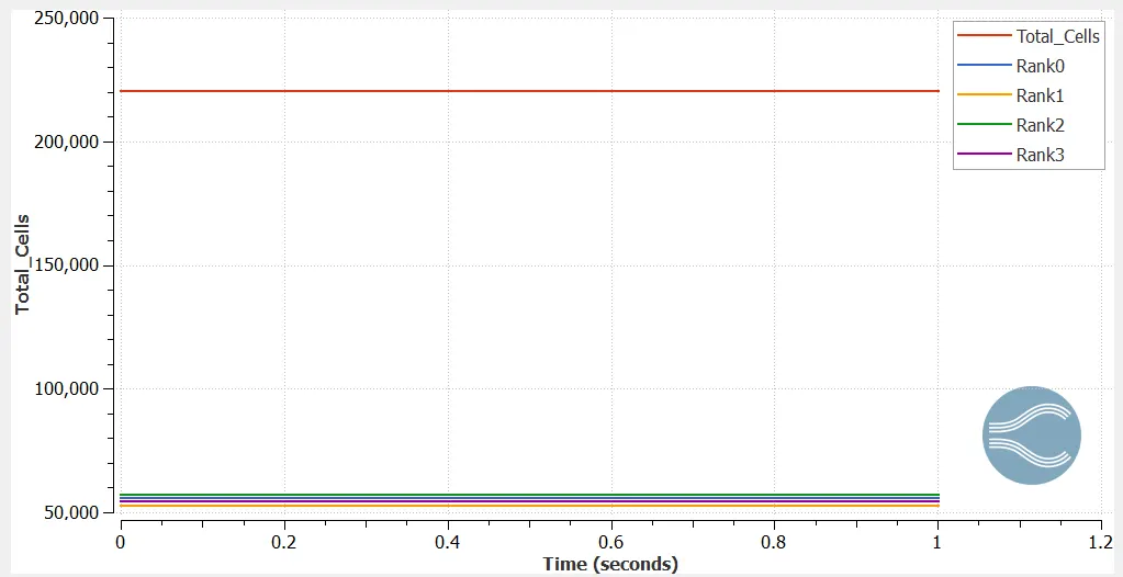
Cell Count Plot
----------------------------------------------------------------------------------------------------------------------
Finding the Coefficient of Lift and Drag using ParaView
ParaView is an important post-processing tool to visualize the results for the FSAE body. Various steps are followed in order to generate Lift and Drag force.
1. First the test.vtm files were imported in Paraview. The .Vtm was created using a converge studio using a post-processing dock.
2. The second step was to generate the Ahmed body so that the "Extract Block" Filter was used to generate the Ahmed body.
3. The third step was to generate the Surface of the FSAE body so a filter called "Extract surface" was used to extract surface for creating the surface normals.
4. Then the surface normals were created using the option in the filter.
5. Then the Lift and Drag force value was calculated using a Virtual calculator.
Lift Force(For single-cell) =PRESSURE*Normals_Z
Drag Force(For single-cell)=PRESSURE*Normals_X
6. Then the cell data were integrated using a filter called "Integrate Variable"
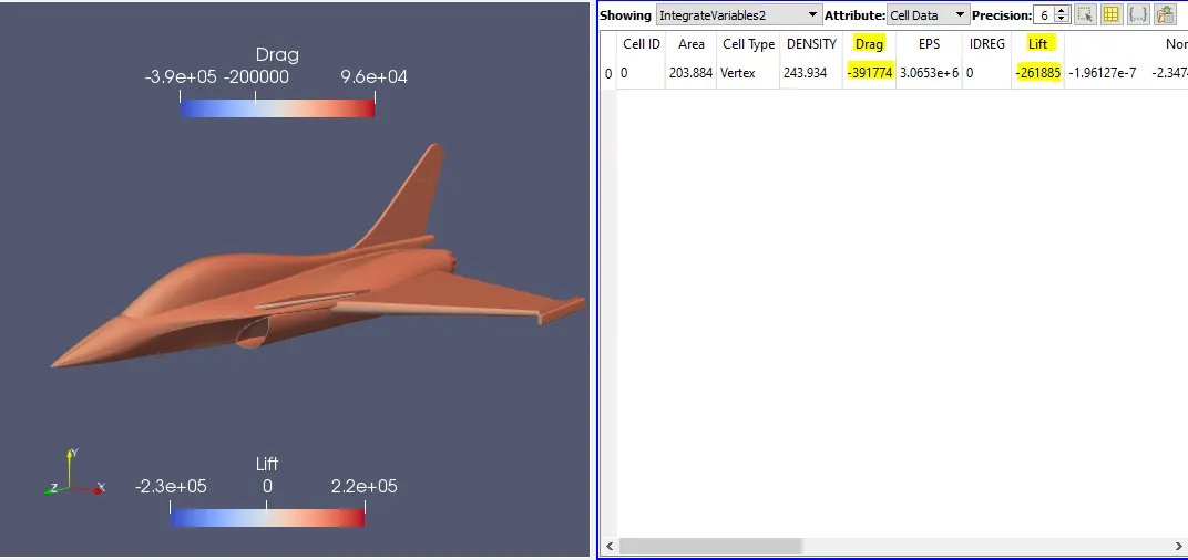
Over All Result For Drag and Lift Force
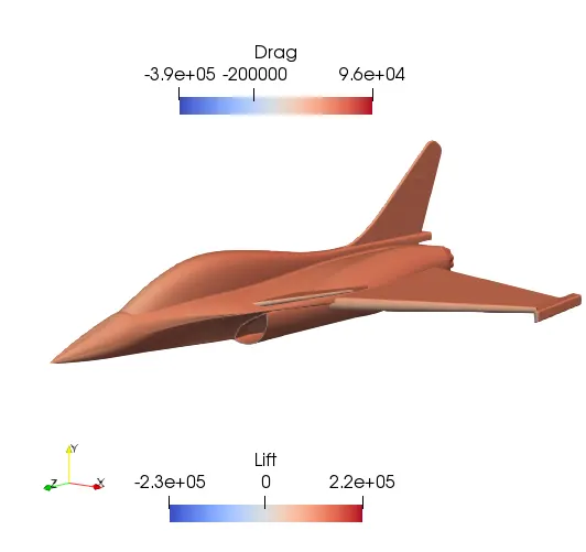
Result
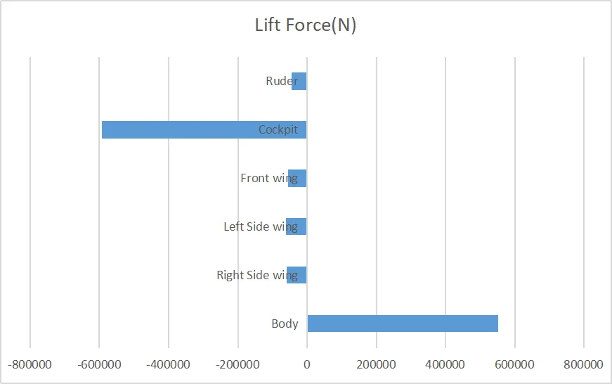
| Lift Force | -261885N |
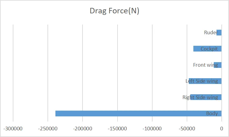
| Drag Force | -391774N |
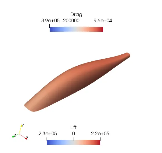
--------------------------------------------------------------------------------------------------
Lift Force Comparison
Drag Force Comparsion
The Case Study can be downloaded from here : Case Study