Steady State Simulation of Tee Mixing Using Ansys
Aim:
The Major Objective of this project was to simulate the flow of air through mixing Tee and Study the effect of length of pipe and momentum ratio of velocity for mixing of air by using two different types of pipe i.e. short and long pipe.
Introduction
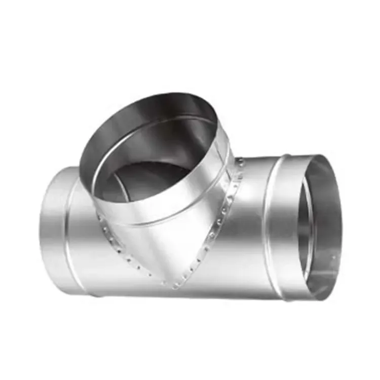
T joints are important flow devices. We can find them in our home mainly Air conditioning applications. It is called T join because it splits the flow and the between them is 90 degrees. A mixing T is useful in getting the desired outlet flow at a particular temperature. The T joint has one Outlet and Two inlets. The major use of Tee joint is in HVAC systems.
The Mixing Effectiveness was compared with different geometry and different momentum ratio.
The hot inlet Temperature was maintained at 36 degrees Celcius whereas the cold inlet is at 19 degrees Celcius.
STEADY STATE SIMULATION:
These are the simulation we run if are just interested in the end result and not in how those results are getting formed with time. The properties do not change with respect to time or there are no time derivative terms in the equations of motion that govern the fluid flow.
If we want to see how results are changing w.r.t time and how the solution is getting formed over time then we need to run the TRANSIENT STATE SIMULATION.
The time is in Cycles for STEADY STATE SIMULATION whereas time is in Seconds for TRANSIENT STATE SIMULATION.
For this project, two different geometry was used and two different case study was run on each geometry with different Momentum Ratio.
The steady-state simulation was performed to compare the mixing effectiveness when the hot inlet temperature is 360C & the Cold inlet is at 190C.
- Case Study 1
- Short mixing tee with a hot inlet velocity of 3m/s.
- Momentum ratio of 2, 4.
- Case Study 2
- Long mixing tee with a hot inlet velocity of 3m/s.
- Momentum ratio of 2, 4.
`"Momentum Ratio"="Velocity at Cold Inlet"/"Velocity at Hot Inlet"`
1.Geometry Creation
First of all, The Tee shaped body geometry was created using a separate CAD package i.e. Solidworks. Then the same geometry was imported in Ansys workbench for generating the fluid flow domain volume to define the boundary conditions and further proceed with Pre Processing, and post-processing the results.
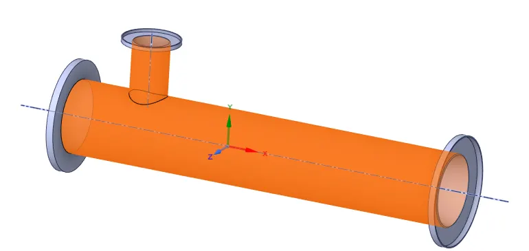
Image 1: CAD model of Tee Geometry
Pre Processing
2. Geometry Creation Using Ansys Design Modular
The Geometry was upload and the fluid region or define the fixed Control Volume was prepared from the option available in Ansys design modular, In order to create the Inlet, outlet, and walls boundary tags easily. this process is sometimes also called Geometry clean up.
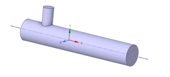
Image 2: Fluid Flow Control Volume.
3. Boundary Creation and Meshing
After the control volumes are perfectly created the boundary tags were created in order to assign the different boundary conditions ie. velocity, temperature, or some other physics. For this geometry, 4 different boundary tags or names were created that were used earlier to assign the boundary condition. The four names are Inlet_X, Inlet_Y, Outlet, and Walls.
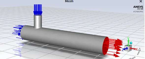
Image 3: Geometry representing the various boundary Tags.
The Blue arrow represents the Inlet, Red color represents the Outlet where the circular walls represent the wall Boundary tag.
Meshing
As the Greomtry was very simple and a simple Tetrahedral Mesh was created using the Automatic Meshing option in Ansys.
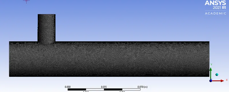
Image 4: Meshed geometry.
Meshing is very important so that for really small infinitesimal control volumes the equation of fluid flow can be used in order to generate useful information.
Mesh Parameters & Information
| Element Size | No. of Elements | No of Nodes | |
| Short Tee Geometry | 1.1e-3m | 456024 | 88086 |
| Long Tee Geometry | 1.3e-3m | 410215 | 79964 |
So the fine mesh was preferred.
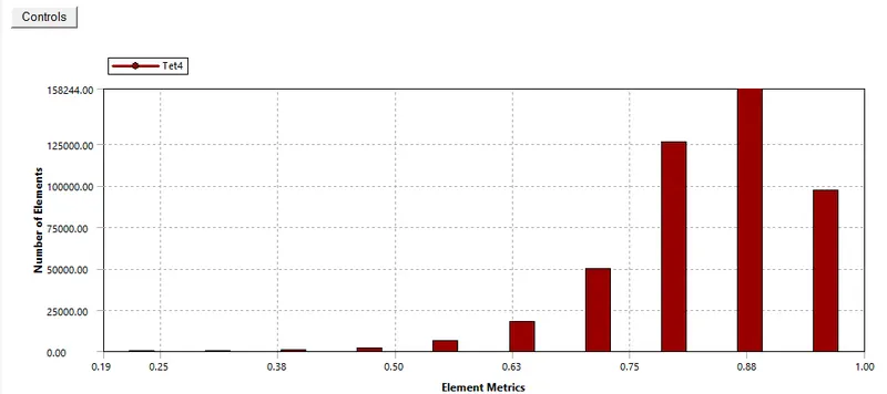
Mesh Quality for Long Tee Geometry
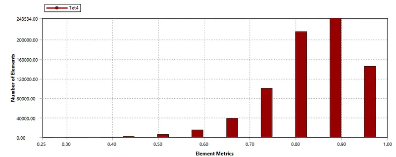
Mesh Quality for Short Tee Geometry
Mesh Independency Test
Mesh independency test was performed in order to use enough elements without compromising with the results and that could help in visualization of mixing flow happening inside Tee geometry.
| Mesh Quality | No of Elements | Outlet Velocity | Outlet Temperature | Comment |
| Coarse(0.003m) | 39393 | 7.1m/s | 290K | The Visualization of the mixing interface was not proper due to the coarse mesh size |
| Medium(1.1e-3m) | 456024 | 6m/s | 300K | The mixing Visualization was excellent as the mesh was fine. |
| Fine (1e-3m) | 656405 | 6m/s | 300K | Had no change in the values. |
4. Case Study Setup
For setting up the case study Ansys Fluent was used in order to simulate the case study.
The various parameter was considered while setup this case study. The case study setup dock was used to set up the problem which appears on the left-hand side of the converge studio
| S.No. | |||
| 1 | Models | Energy Equation | We choose it because we were interested in Temperature plots so energy NS equations need to be solved for this purpose. |
|
Viscous Model-`K-epsilon -"Realizable"` `"Viscous Model"-`K-omega -`sst` |
The turbulence model was used as we were interested in mixing two fluids. | ||
| 2 | Material | Air (N2:O2::23%:77%) | Air was used as the fluid inside the Tee Mixing case study |
| 3 | Cell Zone Condition | Control Volume Region was set to Air | The flow inside the Control volume wanted it to be only air. |
| 4 | Boundary Conditions | Momentum Ratio 2 | Momentum Ratio 4 |
| Inlet X is 3m/s at 360C | Inlet X is 3m/s at 360C | ||
| Inlet Y is 6m/s at 190C | Inlet Y is 12m/s at 190C | ||
| The outlet was set to 0 Guage Pressure | The outlet was set to 0 Guage Pressure | ||
| Walls No slip | Walls No slip |
5. Solution
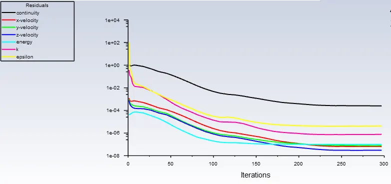
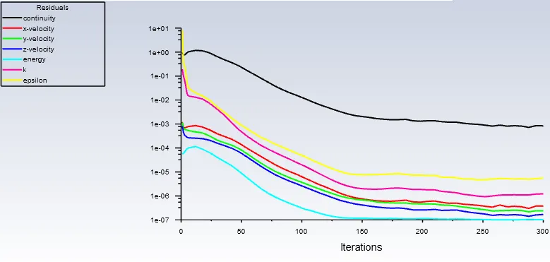
For the Solution Residuals Monitor, the Magnitude was changed to 1e-6 to get less error with more accuracy.
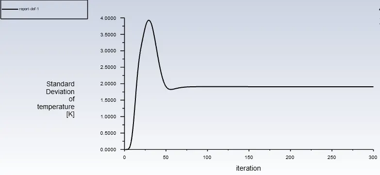
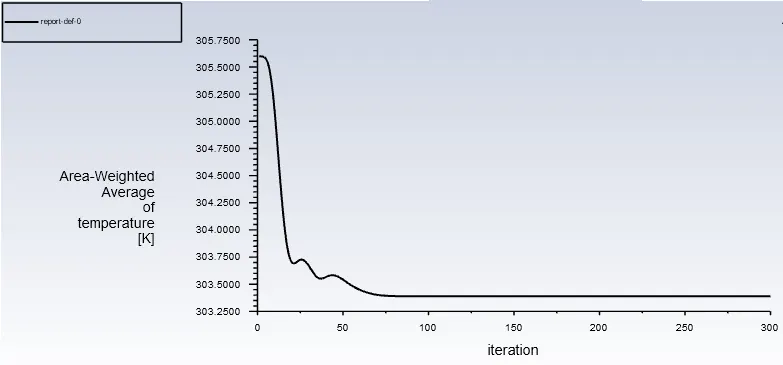
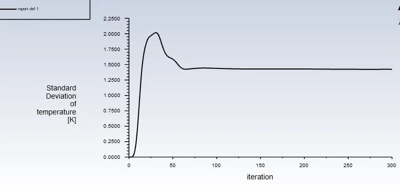
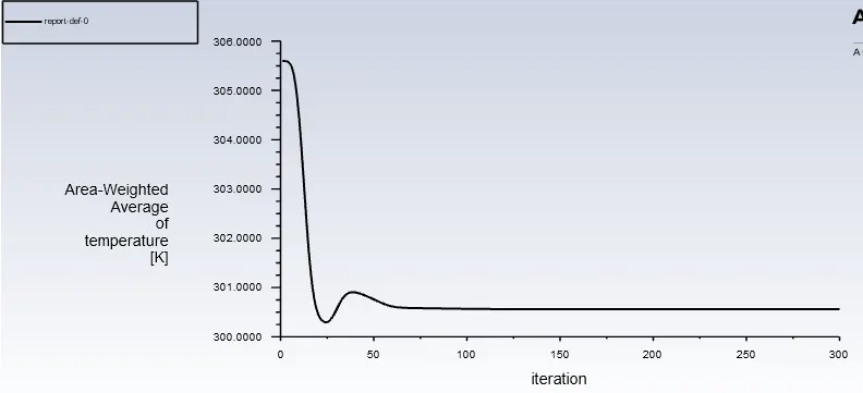
The Surface Report for Temperature at outlet using Standard Deviation and Area Weighted Average.
Hybrid Intilizization was used in order to initialize this simulation.
As this was Steady-State Simulation so the Simulation was run for 300 cycles and the results were generated easily.
Post Processing
Results
Simulation 1:
Long Tee Geometry
Case Study 1: Momentum Ratio 2
| Model Used `K-epsilon -"Realizable"` |
Model Used`K-omega -` sst |
|
Residual Plot
|
Residual Plot
|
|
Area Weighted Report for Temperature at Outlet
|
Area Weighted Report for Temperature at Outlet
|
|
Standard Deviation Report for Temperature at Outlet
|
Standard Deviation Report for Temperature at Outlet
|
|
Temperature Contour
|
Temperature Contour
|
|
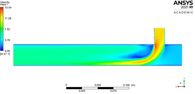
Velocity Contour
|
Velocity Contour
|
|
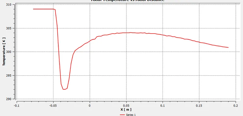
Temperature Versus Axial Distance
|
Temperature Versus Axial Distance
|
|
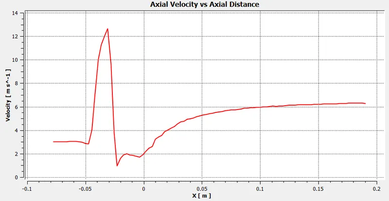
Axial Velocity Versus Axial Distance
|
Axial Velocity Versus Axial Distance
|
|
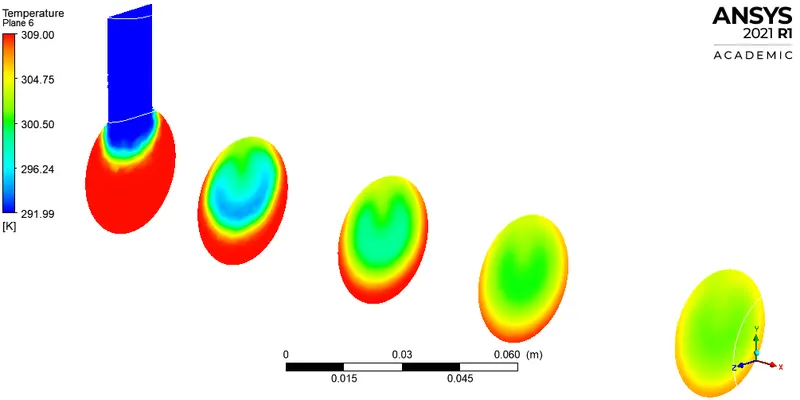
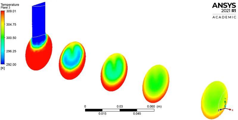
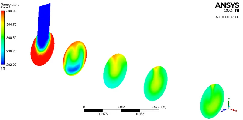
Temperature Contours at different Planes
|
Temperature Contours at different Planes
|
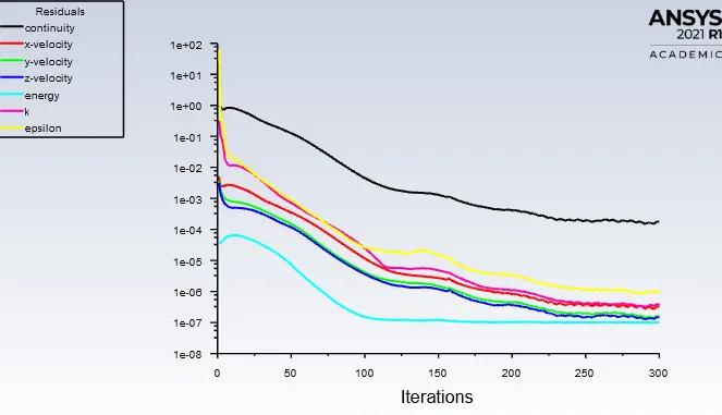
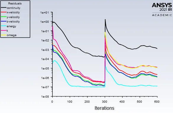
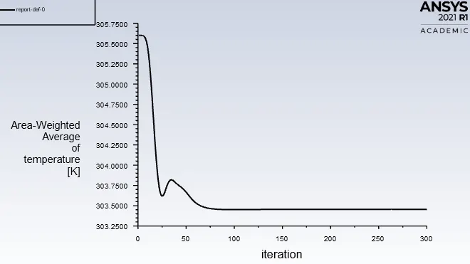
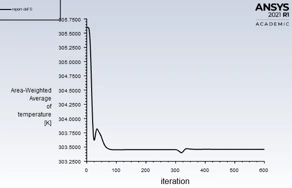
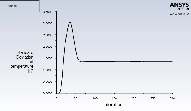
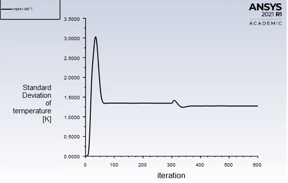
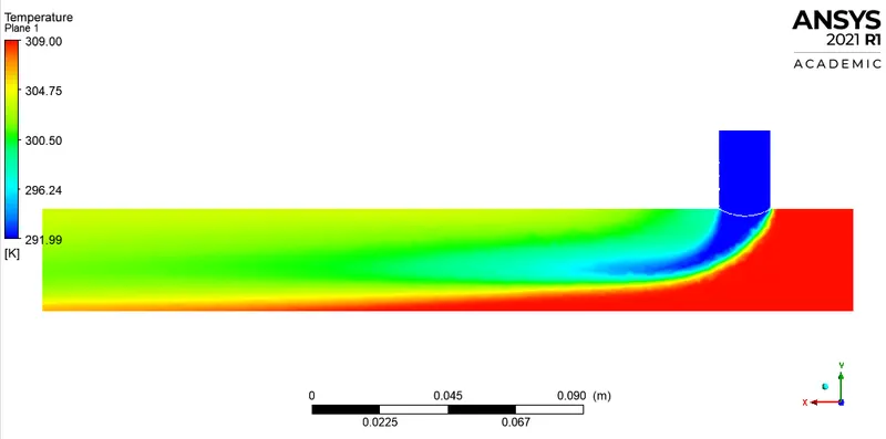
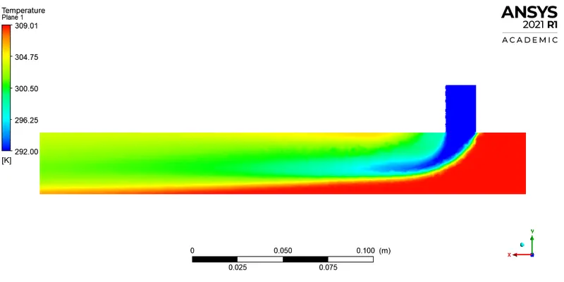
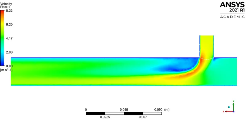
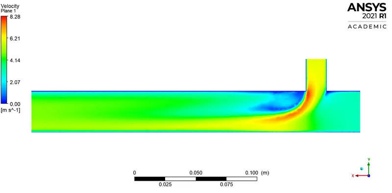
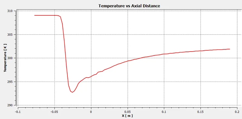
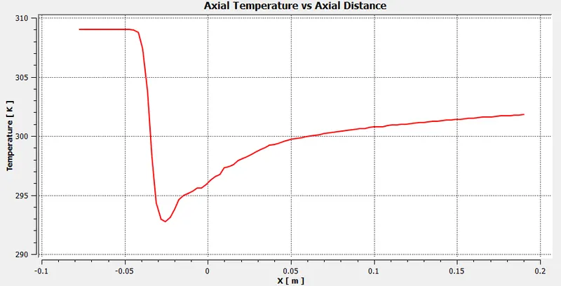
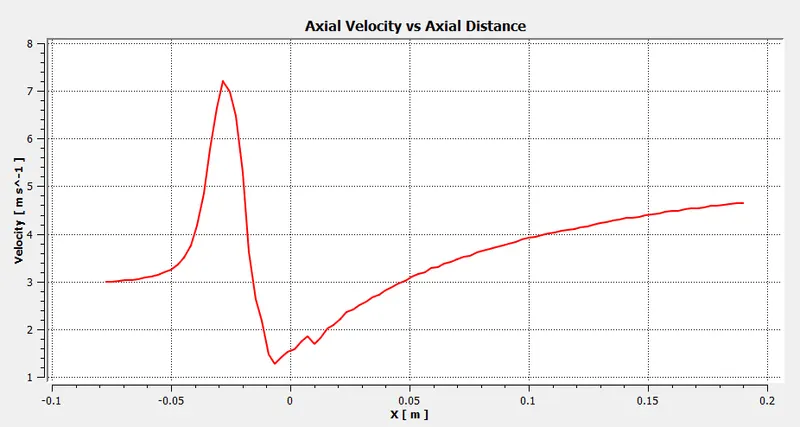
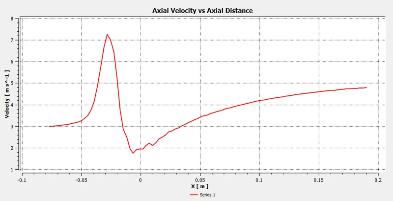
It can easily be observed from the Residual plot that the convergence in the case of `K-epsilon -"Realizable"` is faster and accurate as compared with `K-omega -` sst. So for further Simulations `K-epsilon -"Realizable"` was considered because it provided accurate results within less number of iterations.
Simulation 2:
Long Tee Geometry
Case Study 2: Momentum Ratio 4
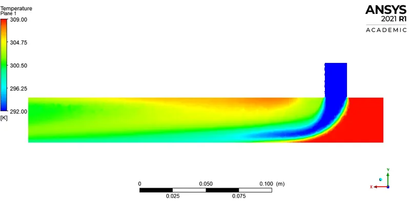
Temperature Contour
Velocity Contour
Temperature Contours at different Planes
Temperature Versus Axial Distance
Axial Velocity Versus Axial Distance
Simulation 3:
Short Tee Geometry
Case Study 1: Momentum Ratio 2
Residual Plots
Standard Deviation Report for Temperature at Outlet
Area Weighted Report for Temperature at Outlet
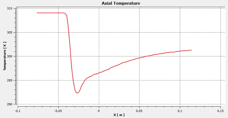
Temperature Versus Axial Distance
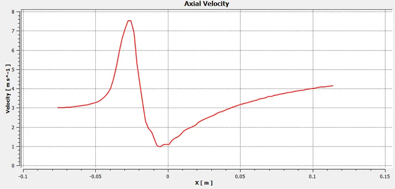
Axial Velocity Versus Axial Distance
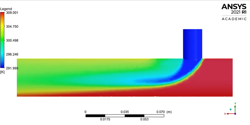
Temperature Contour
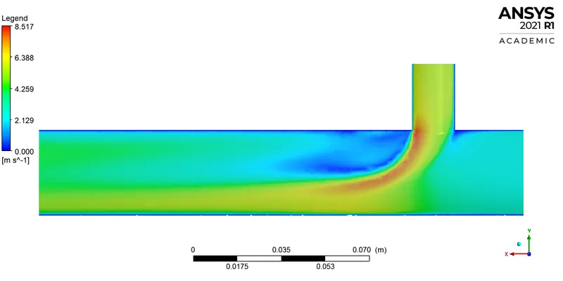
Velocity Contour
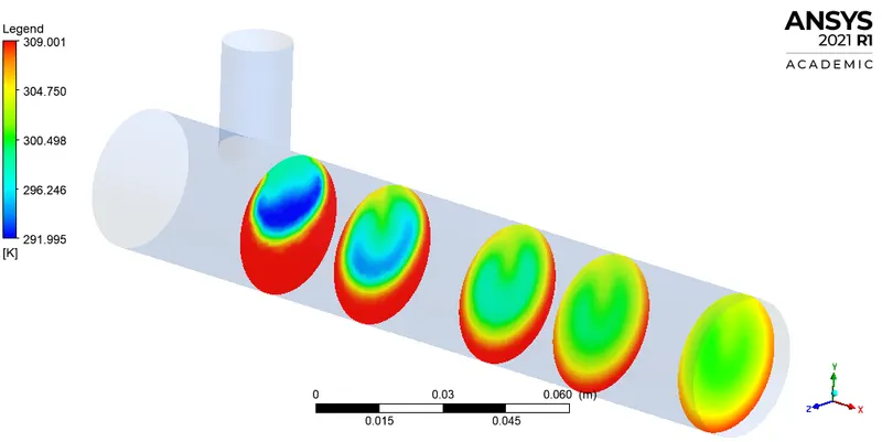
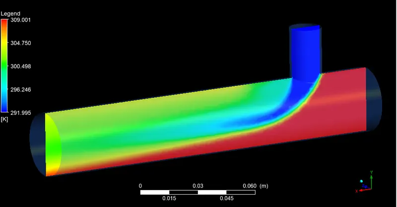
Temperature Contour at Different Planes
Simulation 4:
Short Tee Geometry
Case Study 2: Momentum Ratio 4
Residual Plots
Standard Deviation Report for Temperature at Outlet
Area Weighted Report for Temperature at Outlet
Temperature Versus Axial Distance
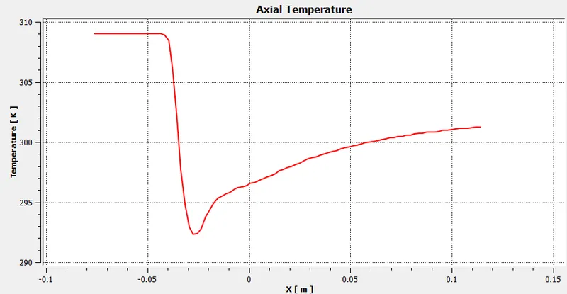
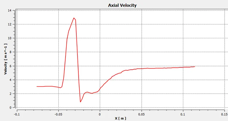
Axial Velocity Versus Axial Distance
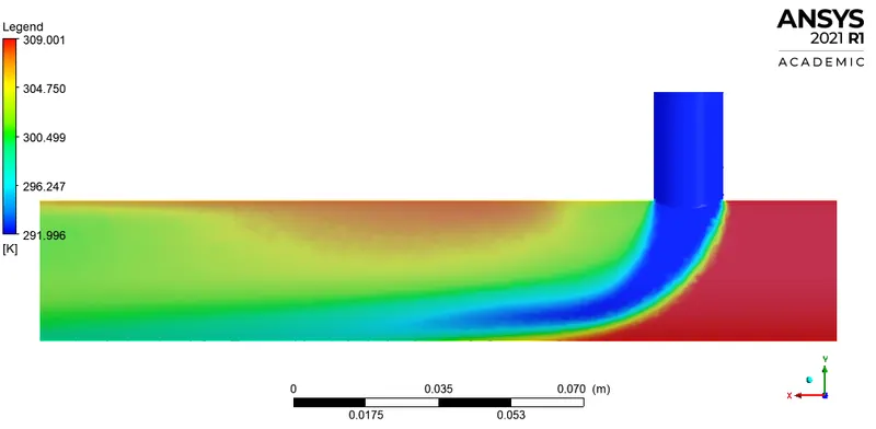
Temperature Contour
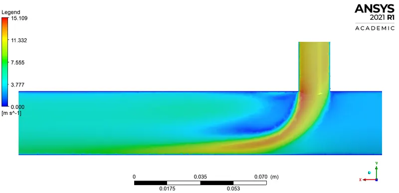
Velocity Contour
Temperature Contour at Different Planes
Conclusion
| Case | No of Elements | Average Outlet Velocity | Average Outlet Temperature | Number of Iterations of Convergence |
| Short Tee-Momentum Ratio 2 | 456024 | 4.1m/s | 303.4K | 198 |
| Short Tee-Momentum Ratio 4 | 456024 | 6.0m/s | 300.6K | 200-220 |
| Long Tee-Momentum Ratio 2 | 410215 | 4.8m/s | 303.3K | 250 |
| Long Tee-Momentum Ratio 4 | 410215 | 6.1m/s | 301K | 200-250 |
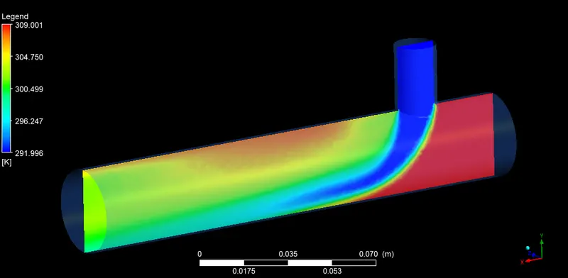
- It can easily be observed that the temperature drop along with uniform mixing in momentum ratio of 4 is more than the momentum ratio 2 in both the case study because the velocity is much higher so air intake is much more that is responsible for effective mixing. This is possible due to turbulent mixing at the Tee joint between hot air and cold air because of the high velocity of cold air which is not possible in the case of low-velocity cold air.
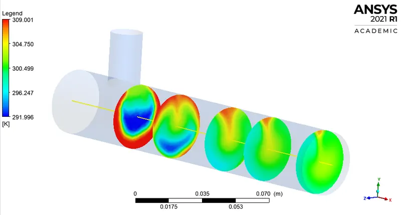
- The temperature contour at different planes clearly explains that the lower the momentum ratio the more low-pressure region at outlet due to improper mixing of air. whereas the case study which has high momentum due to turbulence mixing a uniform temperature distribution can be observed at the outlet patch.
- K epsilon model gave the better results as it predicts well far from boundaries(wall) whereas K -omega model predicts well near the wall. Even though it depends on Y+. therefore, the K-epsilon model is majorly used for free flow away from the wall as in this project, there is no dealing with the wall of mixing tee for change in temperature along the length of it, so k -epsilon model was chosen for simulations.
- It can be concluded that It will be useful to use Tee mixing with long length and High momentum ratio to get effective mixing that ensures uniform results at the outlet.