CHT Analysis on Exhaust port Using Ansys Fluent
Aim:
The main objective was to set up a Steady-State conjugate heat transfer Simulation on the Exhaust port for a four-piston Cylinder Engine using Ansys Fluent and determine the wall heat transfer coefficient.
Introduction:
Conjugate heat transfer is a special case that combines heat transfer in solid and fluid. In the Solid part, conduction dominates whereas fluid part convection dominates. This can be observed in many engineering application like heat exchangers, mufflers cooling ducts, the heat sink is optimized to combine heat transfer by conduction in the heat sink with the convection in the surrounding fluid. Various steps are discussed in this report while making a case set-up for this case study.
Heat transfer in solid is only due to conduction and this is described by Fourier's Law that relates the conductive heat flux(q) is directly proportional to the temperature.
`q=-k nabla T`
whereas time-dependent problem such as transient where temperature field varies with respect to time is given by following partial differential equation:
`rhoC_p (delT)/(delt)=nabla.(knablaT)+Q`
Heat Transfer in a fluid is due to three contribution to the heat equation:
- The transport of fluid implies energy transport too, which appears in the heat equation as the convective contribution. Depending on the thermal properties of the fluid and on the flow regime, either the convective or the conductive heat transfer can dominate.
- The viscous effects of the fluid flow produce fluid heating. This term is often neglected, nevertheless, its contribution is noticeable for fast flow in viscous fluids.
- As soon as a fluid density is temperature-dependent, a pressure work term contributes to the heat equation. This accounts for the well-known effect that, for example, compressing air produces heat.
`rhoc_p (delT)/(delt)+rhoc_pu.nablaT=alpha_pT((delp_a)/(delt)+u.nablap_a)+tau:s+nabla.(knablaT)+Q`
Applications:
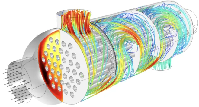
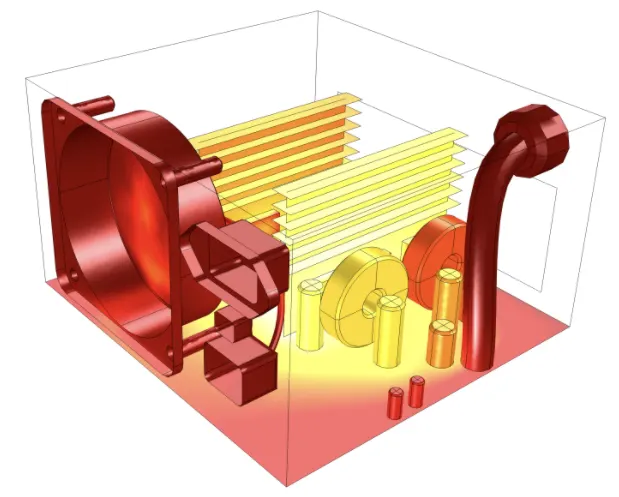
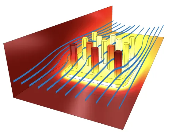
Figure 1 Application of CHT
CHT Modeling Setup
There are several steps to setting up a CHT simulation
1.Define fluid and solid material and their physical properties
2.Configure the fluid and solid regions
3. Assign region to streams.
4. Use appropriate boundary conditions for the boundaries that separated different regions.
5. Select the time control method.
6. Set up post-processing.
Calculation of Grid Size
Y plus Contours
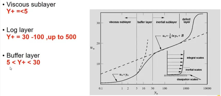
Figure 2. Representation Boundary layer.
Turbulence is the state of chaotic and unstable fluid flow, just opposite of Laminar flow. Y plus(Y+) is the non-dimensional distance of the first cell from the wall.
Let's takes an example of a flat plate under zero pressure gradient and front left side the uniform velocity is coming to the plate. Firstly, it will be laminar flow, then after some disturbance, the region will be called as Transition Region, when the disturbance is growing too much the flow will change in Turbulent Flow. The boundary layer in the turbulent region will be called a turbulent boundary layer whereas in laminar it will be called the laminar boundary layer.
Reynold's Number `Re` is the ratio of Inertial force to the Viscous Force.
Viscous Sub Layer: Viscous stress term dominates
Buffer Layer: Transitional region
Log law Region: Reynolds shear stress term dominates
Reynolds Number Re=55803
The density of Air(at k)=`rho=1.766 frac{kg}{m^3}`
Dynamic Viscosity(at 300k)=`mu =0.00001846 frac{kg}{ms}`
Kinematic Viscosity=`frac{mu}{rho}=1.045 E-05 frac{m^2}{s}`
Pipe Outer Diameter D=0.04m
Average Flow Velocity=`frac{Re*mu}{rho.d}=5 frac{m}{s}`
Skin friction drag coefficient=`Cf=0.0576.Re^frac{-1}{5}=0.006472`
Wall Shear Stress`Tw=Cf.frac{rho.v^2}{2}=0.0983 frac{N}{m^2}`
Frictional Velocity=`ut=sqrtfrac{tw}{rho}=0.2833 frac{m}{s}`
Assuming the desired `y+=32`
Then first cell center to boundary distance=`Y+.frac{v}{ut}=0.00118m=1.18mm`
Cell Size=`2*0.00118*1000=2.36mm`
Geometry Creation:
The Exhaust Geometry was designed using a separate cad package using Solidworks. Then the geometry was imported to Ansys design modular for future control volume creation as it defines the fluid flow domain important for solid and fluid interaction. The Shared Topology option was enabled to create a common geometry with two different phases for the solid and fluid interface. The fluid flow domain was prepared using the volume preparation option in fluent.
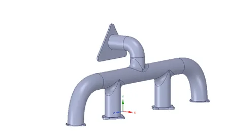
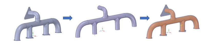
Figure 3. CAD geometry preparation in Ansys Design Modular.
2. Boundary Creation and Meshing
After the control volumes are perfectly created the boundary tags were created in order to assign the different boundary conditions ie. velocity, temperature(if needed), or some other physics. For this geometry, 4 different boundary tags or names were created that were used earlier to assign the boundary condition. The four names are Inlet, Temperature walls, Outlet, and No-slip walls(Adiabatic walls).
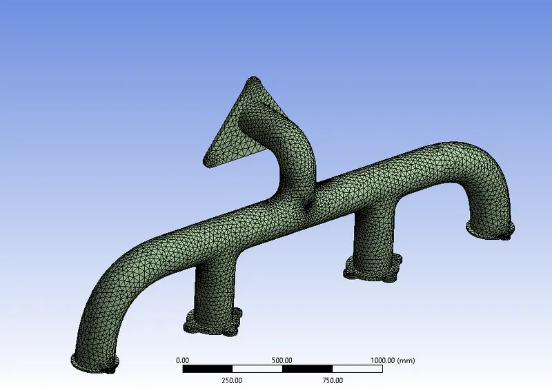
Figure 4. Meshed geometry using 10 mm Base mesh was generated for complete geometry.
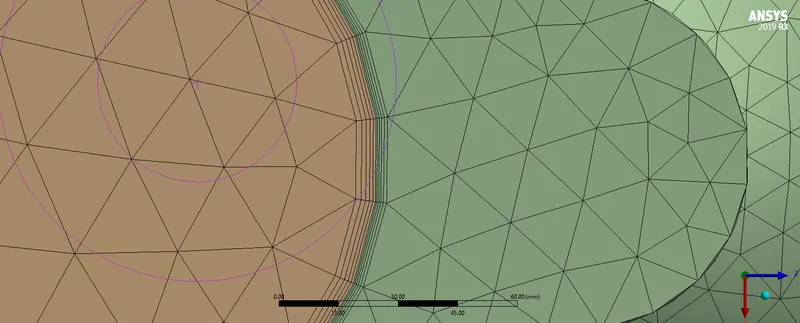
Figure 5. Geometry with inflation layer near to walls.
Inflation layers were added near to the fluid domain to capture the Wall heat flux coefficient more accurately.
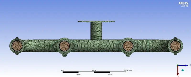
Tet Shape mesh was generated as the flow was not aligned and especially the flow was turbulent.

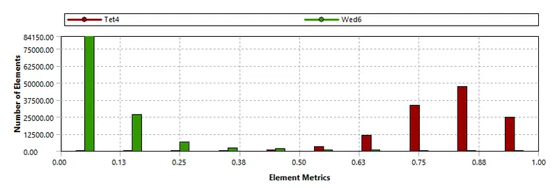
Figure 6. Quality Matrix
3. Case Study Setup
For setting up the case study Ansys Fluent was used in order to simulate the case study.
The various parameter was considered while setup this case study. The case study setup dock was used to set up the problem which appears on the left-hand side of the converge studio
Solver type: Pressure Based Steady State simulation
| S.No. | |||
| 1 | Models | Viscous Model-`K-epsilon -"Standard"` | The turbulence model was used as the inlet velocity was too high therefore Reynolds number was in the turbulent category. |
| 2 | Material |
Air (N2:O2::23%:77%) |
Air was used as the fluid inside the Virtual Wind Tunnel |
| 3 | Cell Zone Condition |
Control Volume Region was set to Air The solid part was set to Aluminium |
The flow inside the Control volume wanted it to be only air. |
| 4 | Boundary Conditions | Inlet X is 5m/s at 700K | |
| The outlet was set to 0 Guage Pressure | |||
| The outer casing of exhaust Walls was convection | 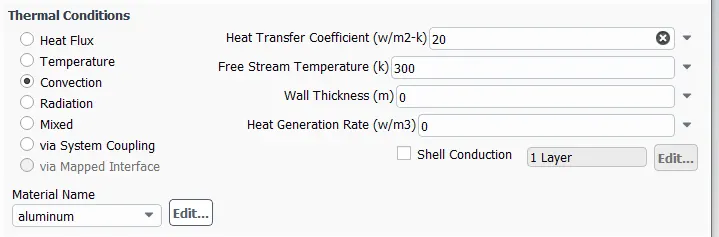 |
||
| The remaining walls were set to adiabatic no-slip walls. |
4. Solution
For the Solution Residuals Monitor, the Magnitude was changed to 1e-6 to get more accuracy.
Hybrid Intilizization was used in order to initialize this simulation.
As this was Steady-State Simulation so the Simulation was run for 500 cycles and the results were generated easily.
Post Processing
Results
Residual Plots
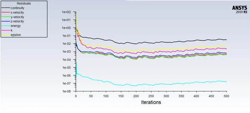
Figure 7. Residual plot for NS equations.
Post Processing -Results
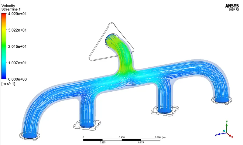
Figure 8. Streamlines representations.
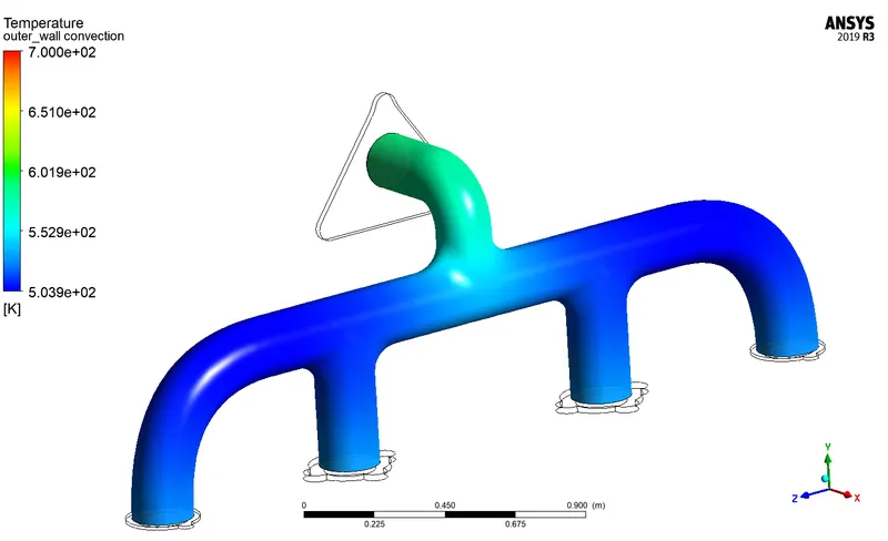
Figure 9. The temperature inside the fluid domain.
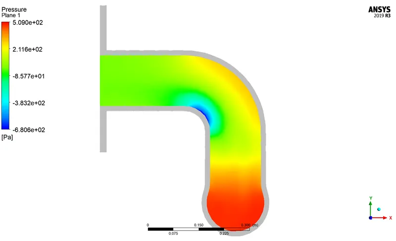
Figure 10. Pressure contour.
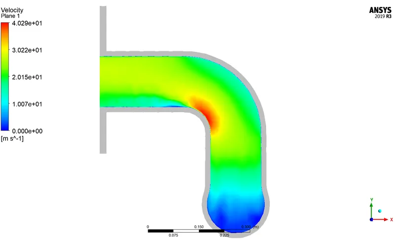
Figure 11. Velocity contour.
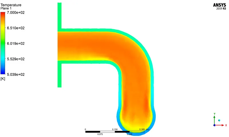
Figure 12. Temperature Contour.
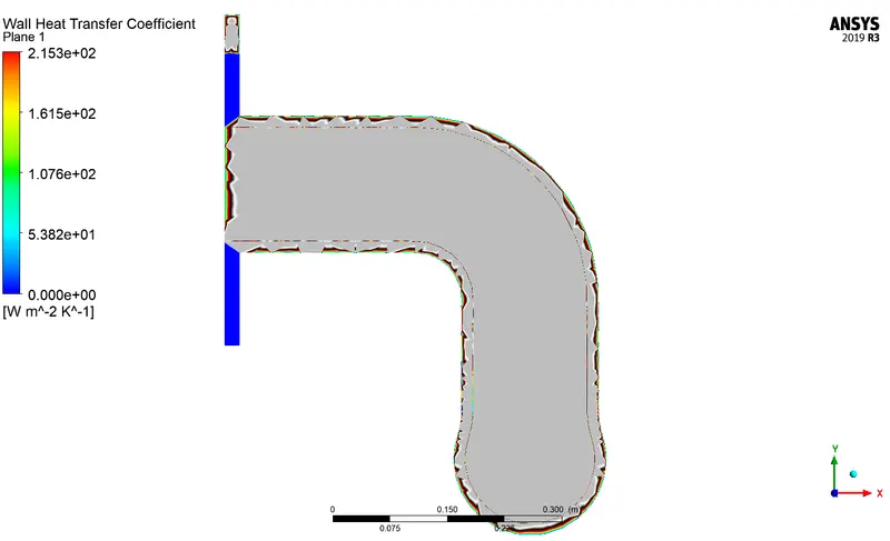
Figure 13. Wall heat Transfer contour.
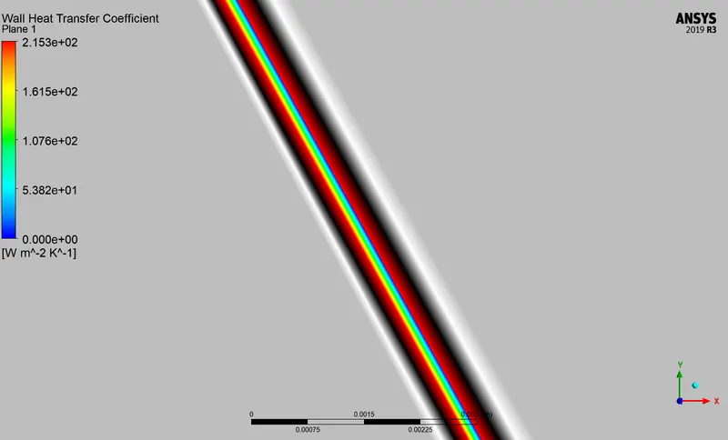
Figure 14. Wall heat Transfer contour.
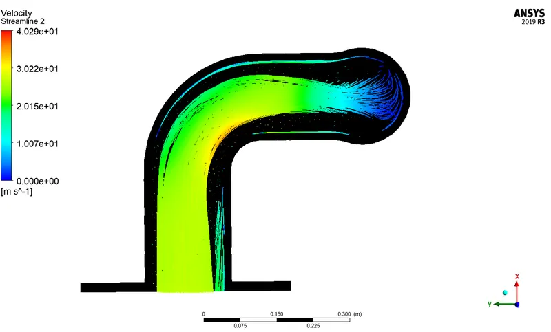
Figure 15. Temperature plus streamlines contour.
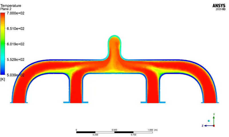
Figure 16. Top temperature contour.
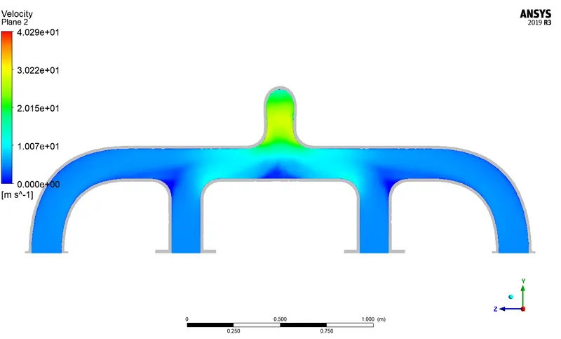
Figure 17. Top Velocity contour.
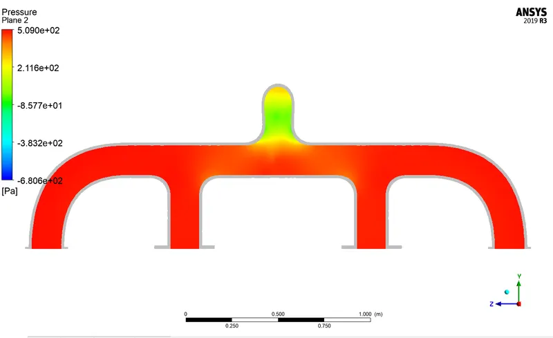
Figure 18. Top Pressure contour.
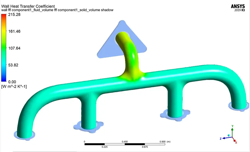
Figure 19. Wall heat transfer coefficient.
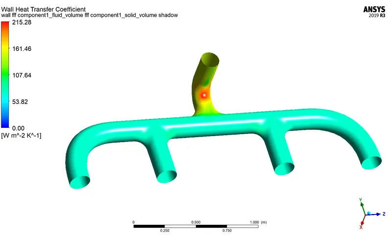
Figure 20. Wall heat transfer coefficient.
Conclusion
Theoretical Calculation for Heat flux Coefficient
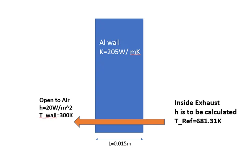


`q=h(T_(wall)-T_(ref))`
`h=1/R`
`q=(T_(wall)-T_(ref))/R`
`R=("Convection resistance")_(out)+"Wall conductivity resistance"+"Convection Resistance"_(Inside)`
`R=(1/h_(out)+L/K+1/h_(In))`
`R=(1/20+0.015/20`R=(DT)/q`5+1/h_(In))`
`q=215 W/(m^2K)`
| Calculated Result | CFD Result | Error % | |
| Wall Heat Transfer Coefficient`W/(m^2K)` | 215 | 215.3 | 0.139% |
Observation:
The velocity, Pressure and wall heat transfer coefficient was found to be maximum near to the end of the bend wall.
The outlet velocity can be found using a continuity equation or conservation of mass:
`A_1V_1+A_2V_2+A_3V_3+A_4V_4=A_oV_o`
`V_("Outlet")=4*0.175^2*5/(0.150^2)`
`V_("Outlet")=27.2m/s`
| Calculated Result | CFD Result | Error % | |
| Outlet Velocity m/s | 27.2 | 25.78 | 5.5% |
Factors on which the result are highly dependent are:
1. Selecting proper base mesh size.
2. Correct application of boundary condition and viscous models.
3. Mesh refinement at particular regions by adding inflation layers to capture the heat flux coefficient accurately.
4. Selecting an accurate solver and scheme.
| Minimum Temperature (K) | 503 |