Solving 1D Linear Convection Using Matlab

Aim:

The major objective of this project was to solve the 1D Convection equation using Matlab and compare the original and final velocity profiles when we change the value of the number of nodes.

Introduction

`frac{delu}{delt}+cfrac{delu}{delx}=0`

The equation above represents the 1D linear equation and its one dimension as it has derivative with respect to x. It a partial differential equation of order and degree as one.

Assumption

1. The domain length is L = 1m

2. The initial velocity profile is a step function. It is equal to 2m/s between x= 0.1 and 0.3 and 1m/s everywhere else.

3. Constant Velocity, C = 1

4. Set time step = 0.01

The program was solved using first-order forward differencing for the time derivative and first-order backward/rearward differencing for the space term.

The effect on Changing the Number of Nodes on the results

Code for Time Marching

for k=1:nt
        for j=2:n(i)
            u(j)=uold(j)-(c*(dt/dx)*(uold(j)-uold(j-1)));
        end

Matlab Code

All the parameters that were mentioned above were used during the Simulation. A total of 3 for loops were used during programming for this problem. The "i" loop was to keep track of the plot for different values of the base grid whereas k and j were to generate the values for the plot using the time marching method the code is given above.

clear all
close all
clc

%Input Parameter

L=1; %Domain length
c=1; %Convective Coefficient

n=[20,40,80,160]; % no of Nodes

t=0.4 %Total Time

dt=0.01 %Time Step

nt=t/dt;

x_sw=0.1; %Start point of Square Wave
x_ew=0.3; %End point of Square Wave

for i=1:4
    x=linspace(0,L,n(i));
    dx=L/(n(i)-1);
    
    u=ones(1,n(i));
    
    n_s(i)=round((x_sw/dx)+1);
    n_e(i)=round((x_ew/dx)+1);
    
    u(:,n_s(i):n_e(i))=2 %Implimenting the Start and End Value that is 2m/s
    uold=u;
    uinitial=u;
    
    for k=1:nt
        for j=2:n(i)
            u(j)=uold(j)-(c*(dt/dx)*(uold(j)-uold(j-1)));
        end
        uold=u;
        
        %plotting the Plots
        figure(i)
        plot(x,uinitial,'color','b')
        hold on
        plot(x,u,'color','g')
        xlabel('Length')
        ylabel('Velocity')
    end
    
    
end

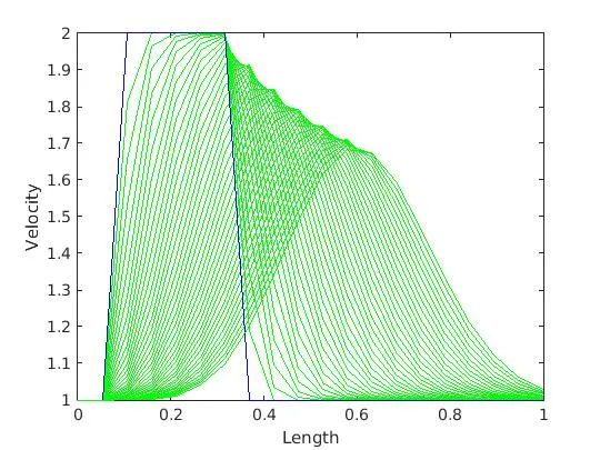
This plot was plotted when the number of nodes is n=20, it can be concluded that there is a little fall or decrease in the velocity profile. The Amplitude of the Velocity keeps on decreasing with the length

The minimum Velocity was found to be between 1.65 m/s to 1.7 m/s.

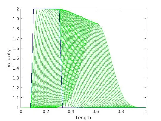
This plot was plotted when the number of nodes is n=40, it can be concluded that there is a very little fall or decrease in the velocity profile as compared to the above result the velocity amplitude is little more. The Amplitude of the Velocity keeps on decreasing with the length

The minimum Velocity was found to be between 1.85 m/s to 1.9 m/s.

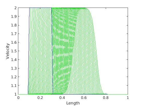
This plot was plotted when the number of nodes is n=80, there is approximately no fall in amplitude in the velocity as it can be seen that the velocity is not decreasing over the domain length and the amplitude remain constant for the domain.

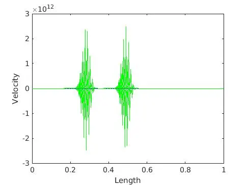
When the grid size is increased then there is a lot of disturbance that can be seen in the result. we see that there is a blow and ripples are formed that make the plot as unstable.

Conclusion

At Last, it can be concluded that as the base grid increases we are near to more accurate results, but if we go beyond some value of the particular grid then that leads to ripples and the results are unstable.