Solving 1D Linear Convection Using Matlab & Studying the effect of Time Step Size

Aim:

The major objective of this project was to solve the 1D Convection equation using Matlab and compare the original and final velocity profiles when we change the Values for the time step.

Introduction

`frac{delu}{delt}+cfrac{delu}{delx}=0`

The equation above represents the 1D linear equation and its one dimension as it has derivative with respect to x. It a partial differential equation of order and degree as one.

Assumption

1. The domain length is L = 1m

2. The initial velocity profile is a step function. It is equal to 2m/s between x= 0.1 and 0.3 and 1m/s everywhere else.

3. Constant Velocity, C = 1

4. Set time step = 0.01

The program was solved using first-order forward differencing for the time derivative and first-order backward/rearward differencing for the space term.

The effect on Changing the Time Step Size on the results

Code for Time Marching

for k=1:nt
        for j=2:n(i)
            u(j)=uold(j)-(c*(dt/dx)*(uold(j)-uold(j-1)));
        end

Code to Print the Plots

plot(x,u,'linewidth',1);
hold on 
axis([0 1 1 2]);
xlabel('Position');
ylabel('Velocity');
title('Effect of time step size on the time marching solutions for explicit schemes'); 
end
plot(x,u_intial,'black','linewidth',2)
 legend('Time step - 0.1','Time step - 0.01','Time step - 0.001','Time step - 0.0001','Original velocity profile')

Two plots commands are being used the first command is to plot the velocity profile using different timesteps whereas the other plot command is used to plot the original velocity.

Matlab Code

The code was made similar with respect to the previous program the different dt values were used to obtain the result the Time marching scheme is mentioned above that was kept in mind while writing the program.

%Important Parameters
L = 1; %length of Domain
n = 80; %base grid size

dt = [1e-1,1e-2,1e-3,1e-4] 
for j = 1:4
 tic
 nt(j)= 0.4./dt(j);
x = linspace(0,L,n);
dx = x(2) -x(1);
c =1;

% Method to define the velocity for the time marching problem
u = ones(1,n);

u(1)= 1;

n_start = 9;
n_stop = 25;
u(n_start:n_stop) = 2 

% Assigning the the velocity at intial time period to the new variable uold
uold = u;
u_intial =u;
%  time =0.4 seconds
% Explicit scheme 
for k =1:nt(j)
 
 for i =2:n
 u(i) = uold(i) -(c*dt(j)/dx)*(uold(i)-uold(i-1));
 end
 uold = u
end
simulationtime(j) =toc
 plot(x,u,'linewidth',1);
hold on 
axis([0 1 1 2]);
xlabel('Position');
ylabel('Velocity');
title('Effect of time step size on the time marching solutions for explicit schemes'); 
end
plot(x,u_intial,'black','linewidth',2)
 legend('Velocity at 0.4 secs -time step - 0.1','Velocity at 0.4 secs -time step - 0.01','Velocity at 0.4 secs -time step - 0.001','Velocity at 0.4 secs -time step - 0.0001','Original velocity profile')

Plot

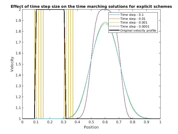
Conclusion

The main thing that can be noticed that the finer the time interval we are closer to the result. as we can clearly see that when we run the program using Time step 0.00001 the velocity profile is approximately close to the original velocity whereas if we talk about time step 0.1 then there is some fall that can be easily noticed in the plot. But the major problem is that the computational time increases as we decrease the Timestep of Simulation. So according to me the cost of computation will increase.