Literature review of Boundary and Initial Conditions
Fluid Flow Equation
2D Incompressible Flow, Newtonian fluid flow and Constant properties
Governing Equation for Boundary Layer
`frac{delu}{delx}+ frac{delv}{dely}=0 -` Continity Equation
`ufrac{delu}{delx}+vfrac{delu}{dely}=-frac{1}{rho}frac{delp}{delx}+v(frac{del^2u}{delx^2}+frac{del^2u}{dely^2})-` X Momentum Equation
`ufrac{delv}{delx}+vfrac{delv}{dely}=-frac{1}{rho}frac{delp}{dely}+v(frac{del^2v}{delx^2}+frac{del^2v}{dely^2})-` Y Momentum Equation
`u frac{delT}{delx}+ vfrac{delT}{dely}=alpha (frac{del^2T}{delx^2}+frac{del^2T}{dely^2})`- Energy Equation
In order to Solve Complex Navier Stokes Equation, The boundary condition plays an important role in making them simple by canceling out some values that would result in achieving pepper results. Selecting proper boundary conditions and initial conditions are very important in order to converge the result. It also a common-sense Question In order to solve let's suppose an ordinary or partial differential equation there must be some boundary condition to find the unknown value of a variable.
Initial Condition
For unsteady problems, we need to specify the value of the variable at time T=0 inside the domain.
General variable
`phi =u,v,w,T,y`
`phi " At time T=0"`
`phi="constant"`
`phi=phi"(x,y,z)"`
Initial condition are very important for steady state problem.
Boundary Conditions
Dirichlet Boundary condition
In Dirichlet Boundary condition, we need to specify the value of the variable at the boundary. It can be constant, varying. and Specialy varying. The value is specified at the boundary
At the Boundary
`phi="constant"`
`phi=phi"(t)"`
`phi=phi"(x,y,z)"`
`phi=phi"(x,y,z,t)"`
Naumann Type Boundary condition
We need to specify the gradient at the boundary or the Flux value that is always normal to the surface
At the Boundary
`frac{delphi}{delx}="constant"`
`frac{delphi}{delx}=0`
`frac{delphi}{delx}=f(t)`
`frac{delphi}{delx}=f(x,y,z)`
`frac{delphi}{delx}=f(x,y,z,t)`
Robin Boundary Condition
It is combination of Dirichlet and Naumann boundary condition thus can we written as
`alphaphi+betafrac{delphi}{delx}=gamma`
Gradient or Flux and value are specified can be clearly seen.
-----------------------------------------------------------------------------------------
Let's Take an Example
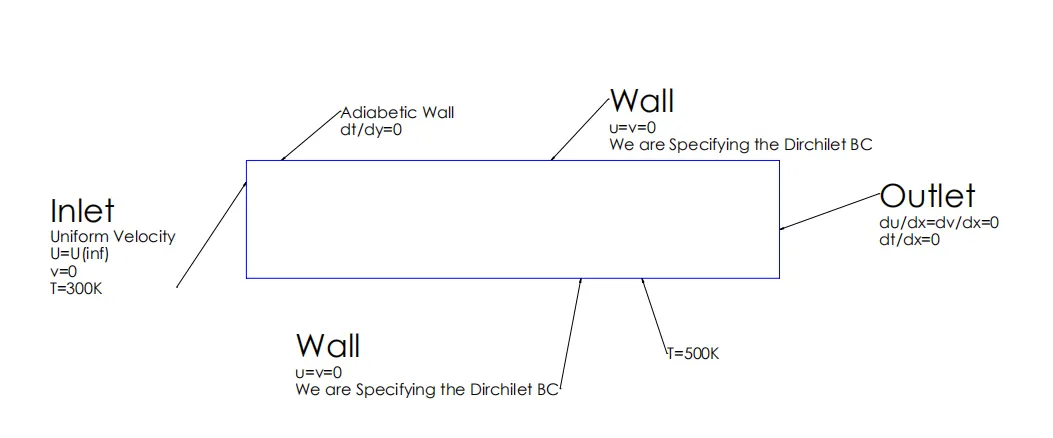
Let us assume that we have two plates that a placed parallel and the Dirichlet type BC are specified at the inlet the fluid is flowing with uniform velocity Uinfinity at 300K. Wall is no slip which means that the velocity of particles near the wall is zero (u=v=0) and the lower plate is maintained at 500K while the other plates are adiabatic wall with heat gradient as zero. the outlet has Naumann type BC.
-------------------------------------------------------------------------------------------
Classification of Partial Differential Equation
In order to solve the PDE, we need to know what kind of PDE that equation is and what BC to apply that plays an important role in solving it.
Type First
Linear
Quasi Linear
Non-Linear
A PDE is linear if the unknown function f(x) and its derivatives appear to the power of 1(Sufficient), It is otherwise a Non-Linear equation. Non Linear if other Function has non linear operator Like f(x)=sin(u)
`frac{delu}{delt}+tfrac{delu}{delx}=0---"Linear"`
`frac{del^2u}{delx^2}+frac{del^2u}{dely^2}=0---"Linear"`
`frac{del^u}{delx}+frac{del^3u}{dely^3}=6ufrac{delu}{delx}---"Non-Linear"`
A PDE is called a quasi-linear if all the terms with highest order derivatives of dependent variables occur linearly, that is the coefficients of such terms are functions of only lower-order derivatives of the dependent variables.
Type Second
First Order
Second Order
Higher-Order
The order of PDE can be easily found using the Maximum derivative that is being used in the PDE.
The Naviour Strokes Equation are generally second order PDE.
`ufrac{delv}{delx}+vfrac{delv}{dely}=-frac{1}{rho}frac{delp}{dely}+v(frac{del^2v}{delx^2}+frac{del^2v}{dely^2})-`2 order PDE'`
`Afrac{del^2u}{delx^2}+Bfrac{del^2u}{dely^2}+Cfrac{del^2u}{delz^2}+D=0`
A,B,C are function of X and Y
D is the function of x,y,u,du/dx,du/dy.
`B^2-4AC<0-"Elliptic"`
Example `frac{del^2T}{delx^2}+frac{del^2T}{dely^2}=0-"Laplace Equation"`
`B^2-4AC=0-"Parabolic"`
Example `frac{delT}{delt}=kfrac{del^2T}{delx^2}--"Heat Equation`
`B^2-4AC<0-"Hyperbolic"`
Example `frac{del^2T}{delt^2}=frac{1}{c}frac{del^2y}{delt^2}--"Wave Equation"`
Type Three
Autonomous
Non Autonomous
Type Four
Homogeneous
NonHomogenous
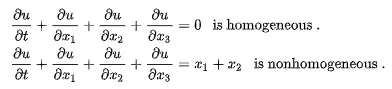
If all the terms of a PDE contain the dependent variable or its partial derivatives then such a PDE is called non-homogeneous partial differential equation or homogeneous otherwise.
Type
Explicit
Implicit